Download
1 / 42
430 likes | 457 Vues
Explore the fundamentals of Cellular Automata including popular models like Wolfram's CA, Conway's Game of Life, Ising Model, Potts Model, XY Model, and Heisenberg Model. Learn about lattice simulations and programming techniques to study these complex systems.

E N D
Cellular Automata What are Cellular Automata or CA? A cellular automata is a discrete model used to study a range of phenomena. These models have applications in: computability theory, mathematics, physics, complexity, biology etc
Cellular Automata CAs generally consist of a grid of cells, each of which has a finite number of possible states. This is what we mean when we say it is a discrete model. The simplest CA cells have two possible states “on” or “off.
Cellular Automata These cells represent the ‘state’ of the simulation. Each cell is updated based on the rules of the CA and the states of the neighbouring cells. This is the ‘dynamics’ of the simulation.
Cellular Automata A Cellular Automata is usually run over many generations to see how the system behaves.
Wolfram’s Cellular Automata One famous Cellular Automata is Wolfram’s CA. This is a one dimensional cellular automata which the value of each cell depends on its state and the state of its two neighbours. These rules can be encoded easily into an integer.
Wolfram’s Cellular Automata Rules for this automata can be easily built from the following representation: This rule set can be represented by the integer 30.
Conway’s Game Of Life Conway’s game of life is an automata designed to simulate life. Each cell in this automata can be either ‘alive’ or ‘dead’.
Conway’s Game Of Life • Any live cell with fewer than two live neighbours dies, as if caused by under-population. • Any live cell with two or three neighbours lives onto the next generation. • Any live cell with more than three live neighbours dies, as if by overcrowding. • Any dead cell with exactly three live neighbours becomes a live cell, as if by reproduction.
Conway’s Game Of Life A simple two-dimensional CA like this can exhibit quite remarkable behaviour. This simple game shows patterns and complex ‘organisms’ emerging from extremely simple rules.
Ising Model The Ising model is model of ferromagnetism named after the physicist Ernst Ising. Each cell in this model represents a magnetic dipole or atomic ‘spins’ in one of two states ‘up’ or ‘down’.
Ising Model Each of these atomic spins interacts with its neighbours and either remains the same or flips. The rules or dynamics of the model are:
Ising Model • If the spin is different to two or more neighbours, change spin. • If the spin is different to zero or one neighbours, change with some probability. • Else remain the same.
Metropolis Algorithm To update this model, iterating through the cells is not acceptable. This causes sweeping effects and the results end up incorrect. Instead we use an update algorithm called the Metropolis Algorithm.
Metropolis Algorithm To update this model, iterating through the cells is not acceptable. This causes sweeping effects and the results end up incorrect. Instead we use an update algorithm called the Metropolis Algorithm.
Metropolis Algorithm Randomly select a spin and compute the energy E(s). Change the spin and calculate the new energy E(s’). Calculate the change in energy ΔE = E(s’)-E(s)
Metropolis Algorithm Accept the change if: ΔE <= 0 or with probability exp(-B*ΔE)
Ising Model Given this update method all we need to define the Ising model is the energy function or Hamiltonian:
Ising Model This is no longer a simple cellular automata because the dynamics depends on some probability. Changing this probability now controls how the model behaves.
Potts Model The Potts model is very similar to the Ising model. However, rather than simply allowing an atomic spin to be ‘up’ or ‘down’ it has Q states. The Potts model with Q=2 is the Ising model.
Potts Model The Potts model is also updated using the Metropolis algorithm, so all we need is the Hamiltonian. The Hamiltonian for the Potts model is simply:
Potts Model This model also shows a phase transition depending on temperature. This is quite an extensible model. Q can be increased to allow each spin to have more possible states. Increase Q enough and this model becomes the XY model.
XY Model The XY model is the extension of the Potts model into continuous space. Rather than a discrete value for each cell, each spin is represented by an angle.
XY Model This model also uses the Metropolis algorithm so all we need is the Hamiltonian:
Heisenberg Model The final extension of this model is the Classical Heisenberg Model where each spin is a three-dimensional vector.
Heisenberg Model Once again this model can be described by a Hamiltonian:
Lattice Simulations These models should show an obvious progression from a simple discrete case of the Ising right through to the more physically realistic Heisenberg Model.
Programming Lattice Simulations Studying these models often requires many simulations and measurements. This is an obvious case when it makes sense to use parallel programming.
Programming Lattice Simulations Task parallelism – The easiest and most obvious way to split up these simulations is to use task parallelism. If you have 1000 simulations to run and 10 machines available. Simply have each machine run 100 simulations and combine the statistics afterwards.
Programming Lattice Simulations This is the best approach if you are using a cluster. Another attractive alternative is to use GPUs. In this case the tasks can’t simply be split between the processors in a GPU because of memory issues.
Programming Lattice Simulations Instead it is better to have each GPU work on one simulation at a time. This is known as data-parallelism. However, for the type of simulation we have discussed there is a significant problem with this: The Metropolis Algorithm
Programming Lattice Simulations Think about the way that the Metropolis Algorithm works. Randomly pick a spin and update it based on the value of its neighbours. If two threads happen to pick spins next to each other, they will update both spins at the same time and update both of them.
Programming Lattice Simulations This may not seem like a big deal but it can have a subtle impact on the behaviour of the simulation. As even a subtle change affects the statistics of the model this is unacceptable.
Programming Lattice Simulations The common solution to this problem is the checkerboard or red/black update method. In this algorithm each cell is colored like a checkerboard. When a model is update, first all the ‘black’ cells are updated and then all the ‘red’ cells are updated.
Programming Lattice Simulations This way no two neighbouring cells are updated at the same time. This is generally accepted to be a suitable solution to the problem.
Programming Lattice Simulations However, it does have an impact on performance. Most memory prediction and caching assumes that sequential memory address will be accessed. This is normally the case for most programs, iterate through a sequence accessing each one.
Programming Lattice Simulations For GPUs this is an even bigger requirement for performance. Sequential threads accessing sequential memory addresses can read all the values in a single transaction, if this condition is not fulfilled the memory reads must be broken into multiple transactions.
Programming Lattice Simulations One method of overcoming this problem is a method called crinkling. This method rearranges the checkerboard so that sequentially access values are stored sequentially.
Programming Lattice Simulations A small change like this can have a large impact on the performance of a simulation.
Summary Cellular Automata Lattice Models Ising Potts XY Heisenberg Metropolis Algorithm Programming Lattice Simulations