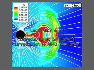
Introduction to Simulations Introduction to MHD Simulation

1. Lectures9 & 10 Introduction to Simulations Introduction to MHD Simulation

2. Categories of Partial Differential Equations • Partial Differential Equations are usually classified into three categories based on the characteristics or curves of information propagation. • Hyperbolic equations – e.g. a wave equation where v=const. is the velocity of propagation. • Parabolic equations- e.g. a diffusion equation where D is the diffusion coefficient. • Elliptic equations – e.g. Poisson equation where r is the source term. For r=0 we have Laplace's equation. • The first two examples are initial value problems – they tell how a system evolves in time and are solved by integrating forward in time. • The third is a boundary value problem - there the system must give the solution everywhere simultaneously. (You can’t integrate in from the boundary like you integrate forward in time). • In global MHD modeling we interested in solving a set of hyperbolic equations at the Sun, heliosphere and magnetosphere and an elliptic equation in the ionosphere.

3. Boundary Value Problems • Stable solutions to boundary value problems are usually easy to achieve. Most effort is on making them efficient. • These become the solution of a number of simultaneous algebraic equations. • Consider a solution to • Represent u(x,y) by its values at specific points where D is the grid spacing • Substitute into the Poisson equation and let uj,l=u(xj.yl)

4. Solutions to Boundary Value Problems • This can be converted into a matrix equation following the prescription in Press (1986) page 618 and the resulting matrix can be inverted. • Define for j=0,1…J, and l=0,1,….,L. In this way i increases most rapidly along the columns representing y values. • The equation now becomes • The points j=0,j=J, l=0, and l=L arethe boundaries where either the function or its derivative are specified. • This gives an equation of the form and can be solved by a number of inversion techniques.

5. A Note on Conservation Laws Consider a quantity that can be moved from place to place. Let be the flux of this quantity – i.e. if we have an element of area then is the amount of the quantity passing the area element per unit time. Consider a volume V of space, bounded by a surface S. If s is the density of the substance then the total amount in the volume is The rate at which material is lost through the surface is

6. Flux Conservation Continued • Use Gauss’ theorem • An equation of the preceding form means that the quantity whose density is s is conserved.

7. Flux-Conservative Initial Value Problems • Many initial value problems can be written in flux-conservative form where u and F are vectors. F is called the conservative flux. • The simplest general flux-conservative equation is the advection equation with a constant velocity v • The solution of this equation is a wave propagating in the positive x-direction where f is some function. • Let's try the most straightforward approach and select equal points in x and t

8. Flux-Conservative Initial Value Problems – The Advection Problem 2 • Forward Euler differencing – First order accurate in time- can calculate quantities at n+1 knowing only previous quantities. • Second order approximation in space using only quantities know at time n. • The resulting approximation in the advective equation called Forward Time Centered Space (FTCS) becomes • Too bad it doesn't work!

9. Flux Conservative Initial Value Problems: Stability • The FTSC approach is an explicit scheme – i.e. ujn+1 can be calculated from things already known. • Assume that the coefficients of the difference equations are slowly varying. In that case the independent solutions (eigenmodes) of the difference equations have the form where k is a real spatial wave number and is a complex number. • The difference equations will have an exponentially growing mode if • The number ξ is called the amplification factor at a given wave number k. • Substitute the equation for ξ into the FTCS equation and get • FTCS is unconditionally unstable because the absolute value of ξ is always greater than one.

10. Flux Conservative Initial Value Problems: The Courant Condition • Let and substitute into the advection equation to give • (Lax Method) • The amplification factor becomes • The stability requirement gives . This is called the Courant-Friedrichs-Lewy stability criterion. Information propagates with a maximum velocity of v. If the differencing scheme requires information from too far away to propagate to a given point it will be unstable. ThereforeDt must not be too large.

11. Flux-Conservative Initial Value Problems: The Courant Condition 2 • How does replacing ujn in the time derivative by its average lead to stable solutions? • Rewrite the equations for the Lax method as • This is the FTCS representation for the equation • The extra term is a diffusion term – we call this adding numerical dissipation or numerical viscosity. • From the amplification factor unless and the wave amplitude decreases. This is better than spurious increases. • Finite-difference schemes also can exhibit dispersion or phase errors. Even if the amplification factor is . At each time step the modes get multiplied by different phase factors depending on their value of k. Eventually the wave packet disperses. • The Lax method is first order in time. Other methods have second order or higher in both time and space. Higher order in time allows larger time steps.

12. Flux-Conservative Initial Value Problems: Shocks and Upwind Differencing • Numerical viscosity tends to control the formation of spurious shocks • In space physics shocks are physically real. • For wave equations propagation (amplitude or phase) errors are usually the most troublesome but for advection transport errors are important. • For example in the Lax scheme j propagates to j+1 and j-1 in the next time step. If v is positive the propagation is only in the plus direction. • One way to deal with transport errors is to use upwind differencing. This uses the fact that depending on the sign of v an advected quantity propagates in one direction. • This is useful where advected variables pass through a shock.

13. An Example of an Implicit Scheme • Consider the parabolic diffusion equation in one spatial dimension • This can be written in flux-conservative form if • Let D be a constant.

14. An Implicit Scheme 2 • Difference it explicitly • Note that the right hand side has a second derivative that has been differenced. • This time the amplification factor is and stability is achieved for • The maximum time step is related to the time it takes to diffuse across the width of a cell or

15. An Implicit Scheme 3 • Since we usually are interested in physical phenomena on scales much larger than Dx this would require us to take too many time steps. • We need to take larger time steps but larger time steps will not work for small scale phenomena. • We might be ok if we could figure out a way to do something that works on large scales at the expense of small scales. • Consider • This is same as before except that everything on the right is at time n+1. • This is an implicit scheme in which you must solve a set of simultaneous equations at each timestep for ujn+1

16. An Implicit Scheme 4 • At large scales the amplification factor becomes • This is unconditionally stable at any time step size! • The details of the small-scale evolution of the initial conditions are inaccurate. • This is first order accurate but higher order schemes are possible. • The biggest drawback of this approach is that you frequently have to invert very big matrices to solve the linear equations. • Some modern approaches combine implicit and explicit approaches. (The solar code used for the flux cancellation model is semi-implicit.) • The two MHD codes we will use in this class are explicit.

17. The Magnetohydrodynamic Equations • Macroscopic plasma properties are governed by basic conservation laws for mass, momentum and energy in a fluid. Mass Momentum Energy* Faraday’s Law Gauss’ Law Ohm’s Law Ampere’s Law • Some solve for a pressure equation

18. Properties of MHD • In ideal MHD the field is frozen-in ( ) provided h is small. • MHD is useful for a wide variety of problems because basically it is a statement of mass, momentum and energy conservation. • Information is propaged by three MHD wave modes. • MHD equations allow us to capture shock waves (important in the supersonic solar wind). • The inclusion of resistivity (h) allows us to break the frozen-in approximation and study magnetic reconnection. • (Outside of space physics MHD equations are used to study dynamos.)

19. MHD wave modes • Alfvén speed: • Sound speed: • Intermediate (Alfvén) wave • Fast and slow waves:

20. Reconnection • As long as frozen in flux holds plasmas can mix along flux tubes but not across them. • When two plasma regimes interact a thin boundary will separate the plasma • The magnetic field on either side of the boundary will be tangential to the boundary (e.g. a current sheet forms). • If the conductivity is finite and there is no flow Faraday’s law and Ampere’s law give a diffusion equation • Magnetic field diffuses down the field gradient toward the central plane where it annihilates with oppositely directed flux diffusing from the other side. • This reduces the field gradient and the whole process stops but not until magnetic field energy has been converted into heat via Joule heating (the resulting pressure increase is what is needed to balance the decrease in magnetic field pressure).

21. Reconnection 2 • For the process to continue flow must transport magnetic flux toward the boundary at the rate at which it is being annihilated. • An electric field in the Ey ( ) direction will provide this in flow. • In the center of the current sheet B=0 and Ohm’s law gives • If the current sheet has a thickness 2l Ampere’s law gives EY JY 2 l EY

22. Reconnection 3 • Equating the EY expressions • Thus the current sheet thickness adjusts to produce a balance between diffusion and convection. This means we have very thin current sheets. • There is no way for the plasma to escape this system. However, if the diffusion is limited in extent then flows can move the plasma out through the sides.

23. Reconnection 4 • When the diffusion is limited in space annihilation is replaced by reconnection • Field lines flow into the diffusion region from the top and bottom • Instead of being annihilated the field lines move out the sides. • In the process they are “cut” and “reconnected” to different partners. • Plasma originally on different flux tubes, coming from different places finds itself on a single flux tube in violation of frozen in flux. • The boundary which originally had Bx only now has Bz as well. • Reconnection allows previously unconnected regions to exchange plasma and hence mass, energy and momentum. • Although MHD breaks down in the diffusion region, plasma is accelerated in the convection region where MHD is still valid.

24. Z X

25. Toward a Self-Consistent Solution

26. Solving the MHD Equations – Magnetospheric Boundary Conditions • The MHD equations are solved as an initial value problem. • Solar wind parameters enter the upstream edge of the simulation and interact with fields and plasmas in the simulation box. • Boundary conditions at the downstream edge, the north and south edges and the east and west edges are set to approximate infinity. • Downstream- where y represents the parameters in the MHD equations. • The bow shock frequently passes through the side and top and bottom boundaries. Here setting the derivative approximately parallel to the shock to zero works well.

27. Magnetosphere Inner Boundary B Ionosphere Solving the MHD Equations: The Inner (Ionosphere) Boundary • Map field aligned currents ( ) from the inner boundary to the ionosphere. • Using current continuity the relationship between the ionospheric potential and the parallel current is • Use mapped FAC and conductivity model to solve for the ionospheric potential F. • For a scalar conductance (S) the potential becomes • This is Poisson's equation and can be solved as a boundary value problem. • Map the potential back to inner boundary and use it to determine boundary condition for the perpendicular flow.

28. Ionospheric conductance • The dense regions of the ionosphere (the D, E and F regions) contain concentrations of free electrons and ions. These mobile charges make the ionosphere highly conducting. • Electrical currents can be generated in the ionosphere. • The ionosphere is collisional. Assume that it has an electric field but for now no magnetic field. The ion and electron equations of motion will be where is the ion neutral collision frequency and is the electron neutral collision frequency. • For this simple case the current will be related to the electric field by where is a scalar conductivity. • If there is a magnetic field there are magnetic field terms in the momentum equation. In a coordinate system with along the z-axis the conductivity becomes a tensor.

29. Specific conductivity – along the magnetic field • Pedersen conductivity – in the direction of the applied electric field • Hall conductivity – in the direction perpendicular to the applied field where and are the total electron and ion momentum transfer collision frequencies and and are the electron and ion gyrofrequencies. • The Hall conductivity is important only in the D and E regions. • The specific conductivity is very important for magnetosphere and ionosphere physics. If all field lines would be equipotentials. • Electric fields generated in the ionosphere (magnetosphere) would map along magnetic field lines into the magnetosphere (ionosphere)

30. Assume a generalized Ohm’s law of the form and that • The total current density in the ionosphere is where and refer to perpendicular and parallel to the magnetic field. • Space plasmas are quasi-neutral so where • The current continuity equation can be written where is along the magnetic field. • Integrate along the magnetic field line from the bottom of the ionosphere to infinity. Since the field lines are nearly equipotentials we can write where the perpendicular height integrated conductivity tensor is

31. Ionospheric Conductance Model • Solar EUV ionization • Empirical model- [Moen and Brekke, 1993] • Diffuse auroral precipitation • Strong pitch angle scattering at the inner boundary of simulation- [Kennel and Petschek, 1966] • Electron precipitation associated with upward field- aligned currents (Knight, [1972] relationship- where FE is the energy flux to the ionosphere, DFis the parallel potential difference, and j is the parallel current density.)

32. Ionospheric Pedersen conductance viewed from dusk. • Note the large day-night asymmetry. This results from ionization by solar EUV radiation.

33. Ionospheric Hall and Pedersen conductance from a simulation of the magnetosphere during a prolonged period with southward IMF. • The white lines show the ionospheric convection pattern. • Precipitation from the magnetosphere enhances both the Hall and Pedersen conductances at night. Pedersen Conductance Hall Conductance

34. Solving MHD Equations: Grids • A wide variety of grids are used. • The grid left is from the model Jimmy Raeder and Mostafa El Alaoui used a non-uniform Cartesian grid. • The BATSRUS code from the University of Michigan uses a Cartesian mesh which is run time adaptive. • Ogino uses a uniform Cartesian grid with 108 cells. • Linker uses a non-uniform spherical grid. • Lyon uses an unstructured spherical grid. • The BATSRUS code from the University of Michigan uses an adaptive mess. • Tatsuki Ogino uses a uniform Cartesian mess with up to 108 grid points.

35. Solving the MHD Equations: Resistivity • The ideal MHD equations are non-dissipative. • Numerical resistivity occurs in all codes caused by the averaging errors inherent in the numerical process. • Most of the MHD modes add dissipation terms to the ideal MHD equations. Some form of dissipation is necessary if phenomena like reconnection, in which ideal MHD breaks down, are to be included in the simulation. • The resistivity models can depend on the physical parameters. For instance in the Raeder-El Alaoui global MHD code the resistivity has a threshold in current density and then is proportional to the currrent density squared ( ).

36. Solving the MHD Equations: Spatial Differencing for Gas Dynamics • A conservative finite difference method to solve the gas dynamics part of the MHD equations. This is the procedure used in the Raeder-El Alaoui code. • The flux-limiting procedure applies diffusion only in the regions where it is necessary to balance dispersive effects.

37. Solving the MHD Equations: Time Stepping • An explicit conservative predictor-corrector scheme for time stepping (second order accurate): • Stability criterion (Courant-Friedrichs-Lewy, CFL): • This must be satisfied everywhere in the simulation domain. • Since characteristic velocity is the Alfvén velocity the Courant condition is important near the Earth where the Alfvén becomes large and the time step becomes small.

38. Solving the MHD Equations: The Field Equations • Place the magnetic field components on the center of the cell faces • Place the electric field components on the centers of the cell edges

39. Divergence of B Control • 8-wave scheme – adds source terms to the MHD equations so that magnetic monopoles are advected with the velocity of the plasma. • Diffusive control – adds the gradient of to the induction equations, so that the error in is diffused away. • Hyperbolic correction adds extra scalar equation to propagate error in with preset speed. • Projection scheme eliminates the errors after each time step by solving a Poisson equation and projecting to a divergence free solution • Constrained transport use a special discretization that the conserves to round off.

40. Some Examples of Global MHD Simulations: The Earth's Magnetosphere • A simulation of the Earth's magnetosphere during a large magnetospheric substorm using the Raeder- El Alaoui code. • The thermal pressure in the noon-midnight meridian plane. • This snapshot was taken at the time of the substorm onset.

41. Some Examples of Global MHD Simulations: Planetary Magnetospheres • The temperature of the plasma in Jupiter's magnetosphere during an interval in which the IMF was northward. • This simulation used the Ogino-Walker MHD code. For this calculation the MHD equations were advanced on a uniform Cartesian grid with ~108 cells. • At Jupiter the model must include atmospherically driven corotation and allow plasma from Io's volcanoes to populate the magnetosphere.

42. Some Examples of Global MHD Simulations: The Heliosphere • The temperature (color spectrogram) and magnetic field lines of an expanding coronal mass ejection. • This calculation was done using the BATSRUS code developed at the University of Michigan. This code uses an adaptive grid.

43. Some Examples of Global MHD Models: Modeling the Sun • Magnetic field lines in the solar corona. • This simulations uses a semi-implicit code developed by Jon Linker and colleagues at SAIC. • The simulation was run on a spherical grid system.