Download
1 / 53
540 likes | 581 Vues
Explore the integration of vision models for comprehensive scene understanding, delving into object detection, depth reconstruction, and multi-class segmentation to interpret complex scenes accurately and efficiently.

E N D
Integrating Vision Models for Holistic Scene Understanding Geremy Heitz CS223B March 4th, 2009
Scene/Image Understanding What’s happening in these pictures?
Human View of a “Scene” BUILDING PEOPLEWALKING BUS CAR ROAD “A car passes a bus on the road, while people walk past a building.”
Computer View of a “Scene” BUILDING Can we integrateall of these subtasks, so that whole > sum of parts ? ROAD STREETSCENE
Outline • Overview • Integrating Vision Models • CCM: Cascaded Classification Models • Learning Spatial Context • TAS: Things and Stuff • Future Directions [Heitz et al. NIPS 2008a] [Heitz & Koller ECCV 2008]
Image/Scene Understanding • Primitives • Objects • Parts • Surfaces • Regions • Interactions • Context • Actions • Scene Descriptions Established techniques address these in isolation. Reasoning over image statistics Man Building Cigarette Backpack Dog Complex web of relations well represented by graphical models. Reasoning over more abstract entities. Sidewalk “a man and a dogare walking on a sidewalkin front of a building”
Why will integration help? What is this object?
More Context Context is key!
Outline • Overview • Integrating Vision Models • CCM: Cascaded Classification Models • Learning Spatial Context • TAS: Things and Stuff • Future Directions [Heitz et al. NIPS 2008a]
Human View of a “Scene” BUILDING • Scene Categorization • Object Detection • Region Labelling • Depth Reconstruction • Surface Orientations • Boundary/Edge Detection • Outlining/Refined Localization • Occlusion Reasoning • ... PEOPLEWALKING BUS CAR ROAD
Related Work • Intrinsic Images • [Barrow and Tenenbaum, 1978], [Tappen et al., 2005] • Hoiem et al., “Closing the Loop in Scene Interpretation” , 2008 • We want to focus more on “semantic” classes • We want to be flexible to using outside models • We want an extendable framework, not one engineered for a particular set of tasks = + =
How Should we Integrate? • Single joint model over all variables • Pros: Tighter interactions, more designer control • Cons: Need expertise in each of the subtasks • Simple, flexible combination of existing models • Pros: State-of-the-art models, easier to extendLimited “black-box” interface to components • Cons: Missing some of the modeling power DETECTIONDalal & Triggs, 2006 DEPTH RECONSTRUCTIONSaxena et al., 2007 REGION LABELINGGould et al., 2007
Cascaded Classification Models Image fREG fDET fREC Features IndependentModels DET0 REG0 REC0 DET1 REG1 REC1 Context-awareModels 3DReconstruction Object Detection RegionLabeling
Integrated Model for Scene Understanding • Object Detection • Multi-class Segmentation • Depth Reconstruction • Scene Categorization I’ll show youthese
Basic Object Detection Detection Window W = Car = Person = Motorcycle = Boat = Sheep = Cow Score(W) > 0.5
Base Detector - HOG • HOG Detector: [ Dalal & Triggs, CVPR, 2006 ] Feature Vector X SVM Classifier
Context-Aware Object Detection • From Base Detector • Log Score D(W) • From Scene Category • MAP category, marginals • From Region Labels • How much of each label is ina window adjacent to W • From Depths • Mean, variance of depths,estimate of “true” object size • Final Classifier Scene Type: Urban scene % of “road” below W P(Y) = Logistic(Φ(W)) Variance of depths in W
Multi-class Segmentation CRF Model • Label each pixel as one of:{‘grass’, ‘road’, ‘sky’, etc } • Conditional Markov random field (CRF) over superpixels: • Singleton potentials: log-linear function of boosted detectors scores for each class • Pairwise potentials: affinity of classes appearing together conditioned on (x,y) location within the image [Gould et al., IJCV 2007]
Context-Aware Multi-class Seg. Where isthe grass? Additional Feature:Relative Location Map
Depth Reconstruction CRF • Label each pixel with it’s distance from the camera • Conditional Markov random field (CRF) over superpixels • Continuous variables • Models depth as linear function of features with pairwise smoothness constraints [Saxena et al., PAMI 2008] http://make3d.stanford.edu
Depth Reconstruction with Context SKY GRASS Sky is far away Grass is horizontal • Find d* • Reoptimize depths with new constraints: BLACK BOX dCCM = argmin α||d - d*|| + β||d - dCONTEXT||
Training ŶS ŶD ŶZ ŶD ŶS ŶZ 0 1 0 1 1 0 I fD fS fZ • I: Image • f: Image Features • Ŷ: Output labels • Training Regimes • Independent • Ground: Groundtruth Input I fD fS fZ ŶS * ŶZ *
Training ŶZ ŶS ŶS ŶZ ŶD ŶD 1 0 1 1 0 0 I • CCM Training Regime • Later models can ignore the mistakes of previous models • Training realistically emulates testing setup • Allows disjoint datasets • K-CCM: A CCM with K levels of classifiers fD fS fZ
Experiments • DS1 • 422 Images, fully labeled • Categorization, Detection, Multi-class Segmentation • 5-fold cross validation • DS2 • 1745 Images, disjoint labels • Detection, Multi-class Segmentation, 3D Reconstruction • 997 Train, 748 Test
CCM Results – DS1 CATEGORIES PEDESTRIAN CAR REGION LABELS BOAT MOTORBIKE
CCM Results – DS2 Boats
Example Results INDEPENDENT CCM
Example Results Independent Objects Independent Regions CCM Objects Independent Objects Independent Regions CCM Regions
Understanding the man “a man, a dog, a sidewalk, a building”
Outline • Overview • Integrating Vision Models • CCM: Cascaded Classification Models • Learning Spatial Context • TAS: Things and Stuff • Future Directions [Heitz & Koller ECCV 2008]
Things vs. Stuff From: Forsyth et al. Finding pictures of objects in large collections of images. Object Representation in Computer Vision, 1996. Thing (n): An object with a specific size and shape. (DETECTIONS) Stuff (n): Material defined by a homogeneous or repetitive pattern of fine-scale properties, but has no specific or distinctive spatial extent or shape. (REGIONS)
Cascaded Classification Models Image fREG fDET fREC Features IndependentModels DET0 REG0 REC0 DET1 REG1 REC1 Context-awareModels 3DReconstruction Object Detection RegionLabeling
CCMs vs. TAS TAS Modeled Jointly CCM Feedforward Image Image fREG fDET fREG fDET DET0 REG0 DET REG DET1 REG1 Relationships
Satellite Detection Example FALSE POSITIVE TRUE POSITIVE
Stuff-Thing Context • Stuff-Thing: • Based on spatial relationships • Intuition: Road = cars here Trees = no cars “Cars drive on roads” “Cows graze on grass” “Boats sail on water” Houses = cars nearby Goal: Unsupervised
Things • Detection TiЄ {0,1} • Ti = 1: Candidate window contains a positive detection ImageWindowWi P(Ti) = Logistic(score(Wi)) Ti
Stuff • Coherent image regions • Coarse “superpixels” • Feature vector Fj in Rn • Cluster label Sj in {1…C} • Stuff model • Naïve Bayes Sj Fj
Relationships • Descriptive Relations • “Near”, “Above”, “In front of”, etc. • Choose set R = {r1…rK} • Rijk=1: Detection i and region j have relation k • Relationship model T1 S72 = Trees S10 = Road S4 = Houses Sj Ti R1,10,in=1 Rijk
Unrolled Model R1,1,left = 1 S1 T1 R2,1,above = 0 S2 R3,1,left = 1 T2 S3 R1,3,near = 0 S4 T3 R3,3,in = 1 S5 CandidateWindows ImageRegions
Learning the Parameters • Assume we know R • Sj is hidden • Everything else observed • Expectation-Maximization • “Contextual clustering” • Parameters are readily interpretable ImageWindowWi K Ti Rijk Sj N Fj J AlwaysObserved AlwaysHidden Supervisedin Training Set
Which Relationships to Use? • Rijk = spatial relationship between candidate i and region j Rij1 = candidate in region Rij2 = candidate closer than 2 bounding boxes (BBs) to region Rij3 = candidate closer than 4 BBs to region Rij4 = candidate farther than 8 BBs from region Rij5 = candidate 2BBs left of region Rij6 = candidate 2BBs right of region Rij7 = candidate 2BBs below region Rij8 = candidate more than 2 and less than 4 BBs from region … RijK = candidate near region boundary How do we avoid overfitting?
Learning the TAS Relations • Intuition • “Detached” Rijk = inactive relationship • Structural EM iterates: • Learn parameters • Decide which edge to toggle • Evaluate with l(T|F,W,R) • Requires inference • Better results than using standard E[l(T,S,F,W,R)] Rij1 Rij2 RijK Ti Sj Fj
Inference • Goal: • Block Gibbs Sampling • Easy to sample Ti’s given Sj’s and vice versa
Results - Satellite Posterior:Detections Prior:Detector Only Posterior:Region Labels
Discovered Context - Bicycles Bicycles Cluster #3
TAS Results – Bicycles • Examples • Discover “true positives” • Remove “false positives” ? BIKE ? ?
Results – VOC 2005 TAS Base Detector
Understanding the man “a man and a dog on a sidewalk, in front of a building ”
Outline • Overview • Integrating Vision Models • CCM: Cascaded Classification Models • Learning Spatial Context • TAS: Things and Stuff • Future Directions