Generative Models for Image Understanding
Generative Models for Image Understanding. Nebojsa Jojic and Thomas Huang Beckman Institute and ECE Dept. University of Illinois. Problem: Summarization of High Dimensional Data. Pattern Analysis: For several classes c=1,..,C of the data, define probability distribution functions p(x| c)

Generative Models for Image Understanding
E N D
Presentation Transcript
Generative Models for Image Understanding Nebojsa Jojic and Thomas Huang Beckman Institute and ECE Dept. University of Illinois
Problem: Summarization of High Dimensional Data • Pattern Analysis: • For several classes c=1,..,C of the data, define probability distribution functions p(x| c) • Compression: • Define a probabilistic model p(x) and devise an optimal coding approach • Video Summary: • Drop most of the frames in a video sequence and keep interesting information that summarizes it.
Generative density modeling • Find a probability model that • reflects desired structure • randomly generates plausible images, • represents the data by parameters • ML estimation • p(image|class) used for recognition, detection, ...
Problems we attacked • Transformation as a discrete variable in generative models of intensity images • Tracking articulated objects in dense stereo maps • Unsupervised learning for video summary • Idea - the structure of the generative model reveals the interesting objects we want to extract.
Mixture of Gaussians c P(c) = pc The probability of pixel intensities z given that the image is from cluster c is p(z|c) = N(z;mc, Fc) z
z p(z|c) = N(z;mc, Fc) Mixture of Gaussians c P(c) = pc • Parameterspc,mc and Fc represent the data • For input z, the cluster responsibilities are P(c|z) = p(z|c)P(c) /Scp(z|c)P(c)
m1= F1= p1= 0.6, m2= F2= p2= 0.4, Example: Simulation P(c) = pc c=1 z= p(z|c) = N(z;mc, Fc)
m1= F1= p1= 0.6, m2= F2= p2= 0.4, Example: Simulation P(c) = pc c=2 z= p(z|c) = N(z;mc, Fc)
Example: Learning - E step P(c|z) c=1 0.52 m1= F1= p1= 0.5, c 0.48 c=2 m2= F2= p2= 0.5, z= Images from data set
Example: Learning - E step P(c|z) c=1 0.48 m1= F1= p1= 0.5, c 0.52 c=2 m2= F2= p2= 0.5, z= Images from data set
Example: Learning - M step m1= F1= p1= 0.5, c m2= F2= p2= 0.5, Set m1 to the average of zP(c=1|z) z Set m2 to the average of zP(c=2|z)
Example: Learning - M step m1= F1= p1= 0.5, c m2= F2= p2= 0.5, Set F1 to the average of diag((z-m1)T (z-m1))P(c=1|z) z Set F2 to the average of diag((z-m2)T (z-m2))P(c=2|z)
Transformation as a Discrete Latent Variable with Brendan J. Frey Computer Science, University of Waterloo, Canada Beckman Institute & ECE, Univ of Illinois at Urbana
Kind of data we’re interested in Even after tracking, the features still have unknown positions, rotations, scales, levels of shearing, ...
Oneapproach Images Labor Normalization Normalized images Pattern Analysis
Ourapproach Images Joint Normalization and Pattern Analysis
What transforming an image does in the vector space of pixel intensities • A continuous transformation moves an image, , along a continuous curve • Our subspace model should assign images near this nonlinear manifold to the same point in the subspace
Tractable approaches to modeling the transformation manifold \ Linear approximation - good locally • Discrete approximation - good globally
Adding “transformation” as a discrete latent variable • Say there are N pixels • We assume we are given a set of sparse N x Ntransformation generating matricesG1,…,Gl,…,GL • These generate points from point
Transformed Mixture of Gaussians P(c) = pc c p(z|c) = N(z;mc, Fc) P(l) = rl l z p(x|z,l) = N(x; Glz, Y) • rl,pc,mc and Fc represent the data • The cluster/transf responsibilities, P(c,l|x), are quite easy to compute x
m1= F1= m2= F2= Example: Simulation G1 = shift left and up, G2 = I, G3 = shift right and up c=1 z= l=1 x=
c l z x ML estimation of a Transformed Mixture of Gaussians using EM • E step: Compute P(l|x), P(c|x) and p(z|c,x) for each x in data • M step: Set • pc = avg of P(c|x) • rl = avg of P(l|x) • mc = avg mean of p(z|c,x) • Fc = avg variance of p(z|c,x) • Y = avg var of p(x-Gl z|x)
Face Clustering Examples of 400 outdoor images of 2 people (44 x 28 pixels)
Mixture of Gaussians 15 iterations of EM (MATLAB takes 1 minute) Cluster means c = 1 c = 2 c = 3 c = 4
Transformed mixture of Gaussians 30 iterations of EM Cluster means c = 1 c = 2 c = 3 c = 4
Video Analysis Using Generative Models with Brendan Frey, Nemanja Petrovic and Thomas Huang
Idea • Use generative models of video sequences to do unsupervised learning • Use the resulting model for video summarization, filtering, stabilization, recognition of objects, retrieval, etc.
c c l l z z x x t-1 t Transformed Hidden Markov Model P(c,l|past)
THMM Transition Models • Independent probability distributions for class and transformations; relative motion P(ct , lt | past)= P(ct | ct-1) P(d(lt , l t-1)) • Relative motion dependent on the class P(ct , lt | past)= P(ct | ct-1) P(d(lt , l t-1) | ct) • Autoregressive model for transformation distribution
Inference in THMM • Tasks: • Find the most likely state at time t given the whole observed sequence {xt} and the model parameters (class means and variances, transition probabilities, etc.) • Find the distribution over states for each time t • Find the most likely state sequence • Learn the parameters that maximize he likelihood of the observed data
c Video summary Image segmentation l z Removal of sensor noise x Image Stabilization Video Summary and Filtering p(z|c) = N(z;mc, Fc) p(x|z,l) = N(x; Glz, Y)
mc 1 class 121 translations (11 vertical and 11 horizontal shifts) Fc mc Fc 5 classes Example: Learning • Hand-held camera • Moving subject • Cluttered background DATA
Examples • Normalized sequence • Simulated sequence • De-noising • Seeing through distractions
Future work • Fast approximate learning and inference • Multiple layers • Learning transformations from images Nebojsa Jojic: www.ifp.uiuc.edu/~jojic
Subspace models of imagesExample: Image, R 1200 = f (y, R 2) Shut eyes Frown
Factor analysis (generative PCA) p(y) = N(y; 0, I) y The density of pixel intensities z given subspace point y is p(z|y) = N(z;m+Ly, F) z Manifold: f (y) = m+Ly, linear
Factor analysis (generative PCA) p(y) = N(y; 0, I) y p(z|y) = N(z;m+Ly, F) • Parametersm,L represent the manifold • Observing z induces a Gaussian p(y|z): COV[y|z] = (LTF-1L+I)-1 E[y|z] = COV[y|z] LTF-1 z z
m = Shut eyes Frown Example: Simulation SE y L = p(y) = N(y; 0, I) Frn p(z|y) = N(z;m+Ly, F) z
m = Shut eyes Frown Example: Simulation SE y L = p(y) = N(y; 0, I) Frn p(z|y) = N(z;m+Ly, F) z
m = Shut eyes Frown Example: Simulation SE y L = p(y) = N(y; 0, I) Frn p(z|y) = N(z;m+Ly, F) z
Transformed Component Analysis p(y) = N(y; 0, I) y p(z|y) = N(z;m+Ly, F) P(l) = rl z l The probability of observed imagex is p(x|z,l) = N(x; Glz, Y) x
m = L = Shut eyes Frown Example: Simulation G1 = shift left & up, G2 = I, G3 = shift right & up SE y Frn z l=3 x
G G a a r r b b a a g g e e Example: Inference G1 = shift left & up, G2 = I, G3 = shift right & up SE SE SE y y y Frn Frn Frn P(l=1|x) = .01 P(l=2|x) = .01 P(l=3|x) = .98 z z z l=1 l=2 l=3 x x x
EM algorithm for TCA • Initialize m, L,F, r, Y to random values • E Step • For each training case x(t), infer q(t)(l,z,y) = p(l,z,y |x(t)) • M Step • Compute mnew,Lnew,Fnew,rnew,Ynewto maximize St E[ log p(y) p(z|y) P(l) p(x(t)|z,l)], where E[] is wrt q(t)(l,z,y) • Each iteration increases log p(Data)
A tough toy problem • 144, 9 x 9 images • 1 shape (pyramid) • 3-D lighting • cluttered background • 25 possible locations
1st 8 principal components: TCA: • 3 components • 81 transformations - 9 horiz shifts - 9 vert shifts • 10 iters of EM • Model generates realistic examples m L:1L:2 L:3 F Y
Expression modeling • 100 16 x 24 training images • variation in expression • imperfect alignment
Factor Analysis: Mean + 10 factors after 70 its of EM TCA: Mean + 10 factors after 70 its of EM PCA: Mean + 1st 10 principal components
Fantasies from FA model Fantasies from TCA model
Modeling handwritten digits • 200 8 x 8 images of each digit • preprocessing normalizes vert/horiz translation and scale • different writing angles (shearing) - see “7”