Download
1 / 29
290 likes | 314 Vues
Learn about MIRIAD, a collection of programs for multichannel image reconstruction, analysis, and display. Understand the different tasks, file types, and documentation available. Explore how to use MIRIAD through the command line and the MIRIAD shell. Discover the basic data reduction procedure, inspecting u-v data, flagging, calibration, and creating maps.

E N D
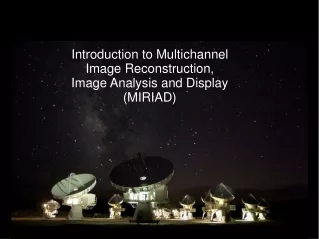
Introduction to Multichannel Image Reconstruction, Image Analysis and Display (MIRIAD)
MIRIAD is a collection of programs or tasks that use a common interface The tasks can be called either directly from the command line or from inside the command shell Both interfaces have their advantages MIRIAD can be used for both u-v data calibration/analysis and image manipulation/analysis General categories of MIRIAD tasks: General Utility Data Transfer Visual Display Calibration uv Analysis Map Making Deconvolution Plotting Map Manipulation Map Combination Map Analysis Profile Analysis Model Fitting Tools Other
What is a MIRIAD file? 2 types of MIRIAD files: u-v data & images MIRIAD files are directories u-v data • “streaming” data • data contains • visdata actual u-v data and preamble • vartable listing of all metadata and data type • header • history listing of what has been done to the data • flags binary flag for every channel in every integration • additional files • calibration tables (e.g. bandpass, gains, leakage) • observing script image data • data contains • image raw image data • header listing of descriptors of the data • history • mostable listing of mosaic parameters • mask flags for individual pixels preamble for each record contains: time stamp (MJD) u,v,(w) baseline lengths in ns baseline number
Documentation Documentation for MIRIAD tasks is generated during compilation You can use doc and mirhelp to access the documentation from command line doc -t $MIRDOC/prog/*.doc lists all tasks by category doc <task> displays the documentation from the given task Additionally there is the MIRIAD manual program: mir.man
Using MIRIAD MIRIAD shell commands: • type miriad in command line to start shell • use inp <task> or tget <task> to open the given task • can type help to get documentation on current task • type <keyword>=<input> to set the variables for the given task • typing inp at any point will refresh the listing • type go to execute the task MIRIAD from the command line • just type the task name along with the inputs (e.g. uvlist vis=c0541.mir options=brief)
Most MIRIAD tasks share common keywords • vis input visibility file(s) • line selection criteria based on channels line=channel|velocity|wide|felocity,<nchan>,<start>,<width>,<step> line=chan,32,1,2,2 will select 32 output channels, averaging every 2 together • select selection criteria based on other parameters some criteria are: time, ra, dec, antenna, window, source, auto they can be combined, separated by commas, a – in front denotes exclusion select=window(2),source(ORIONKL),-auto will select all data from window 2, that is from ORIONKL and is not autocorrelated • options extra processing options passed to the task • in input image file(s) • region selection criteria for images criteria are: images, quarter, box, polygon, mask modifiers include: abspixel, relpixel, arcsec region=arcsec,box(-10,-10,10,10) will select all pixels in a box that is 20” x 20” centered on the reference pixel of the map Note that the antenna selection is special ant(1,2) will select all data from antennas 1 & 2 ant(1,2)(3,4) will select all data from baselines 1-3, 1-4, 2-3 & 2-4
Basic data reduction procedure Inspect the data for obvious errors Flagging “bad” data Calibration: Linelength Passband Gain (amplitude and phase) includes both atmospheric corrections and band phase offsets Create maps: Invert Cleaning the map Inspect maps & spectra There are different routes one can take to producing good maps
Inspecting u-v data listobs gives a good general overview of a track
Inspecting u-v data uvindex gives a more specific overview of a track
Inspecting u-v data varlist lists all u-v header variables in the data set varlist vis=c0541.1C_92OrionK.2.miriad
Inspecting u-v data varplt plots u-v header variables against time (or each other) smavarplt vis=c0541.1C_92OrionK.2.miriad yaxis=systemp device=/xs
Inspecting u-v data uvlist lists different parameters of the data uvlist vis=c0541.1C_92OrionK.2.miriad options=spec,brief
Inspecting u-v data uvplt displays u-v data in graphical format (amplitude/phase vs time/uvdistance) uvplt vis=ori axis=time,amp select=win'(1)',-auto,source'(ORIONKL)' device=/xs Really good data (maser) OK data but some flagging needed
Inspecting u-v data uvspec displays the spectra of the u-v data (amp/phase vs channel) uvspec vis=c0541.1C_92OrionK.2.miriad interval=10000 device=/xs \ axis=chan,amp select=source'(0423-013)'
Flagging uvflag is used to flag/unflag visibilities uvflag vis=temp541 select=time'(02:23:23,02:33:48)' flagval=flag
Passband calibration As the astronomical signals transit to the correlator a frequency dependent phase and amplitude shifts are induced on the signal. Most of this is due to the hardware (filters, fiber lengths, etc) However a small fraction is due to the atmosphere. There are several ways to correct for this: • Use an astronomical source with no spectral features (e.g. quasar) • Use the internal noise source • Use the auto-correlations
Passband calibration Example: using the noise source Since the noise source is only in the LSB we must conjugate the data to create the USB signal using uvcal: uvcal vis=noise options=noisecal out=noise.conj mfcal is used to solve for the passband correction mfcal vis=noise.conj interval=99999 line=chan,952,1,1,1 refant=9\ tol=0.001 Use gpcopy to copy the bandpass from the bandpass calibrator to the source and other calibrators gpcopy vis=noise.conj out=source options=nocal
Passband calibration For auto-correlations use uvcal with options=fxcal For astronomical sources the procedure is similar to the noise source Depending on the correlator setup one may need to bootstrap some solutions e.g. use the wide windows to correct for the atmospheric passband for the narrow windows Use uvcat to apply the gains to the data, otherwise future gains will overwrite the most recent ones uvcat vis=c0541.1C_92OrionK.2.miriad out=c0541.lc
Gain calibration There are two quantities solved for in gain calibration: amplitude gain and phase gain To get the flux of your calibrator there are several methods: 1. If a flux calibrator was observed (planets are primary, quasars are secondary) separate out the flux cal and gain cal (using uvcat) selfcal on these source (more on selfcal in a minute) use bootflux to determine the flux bootflux vis=uranus,0423-013 line=chan,1,1,952,952 taver=15 \ primary=uranus 2. If no flux calibrator was observed the selfcal routines can look up the flux for you or you can look up recent values for your calibrator from the CARMA calibrator web page: http://carma.astro.umd.edu/cgi-bin/calfind.cgi
Gain calibration Self calibration – corrects the data for phase and amplitude fluctuations due to the atmosphere mselfcal can be used for this mselfcal vis=c0423-013 interval=5 options=apriori,noscale \ refant=9 flux=5.9 line=chan,1,1,63,63 Then use gpcopy to apply the gains to the source
Other useful tasks uvcat - copies data to a new file useful for separating individual sources, windows, time ranges etc. can apply gains and bandpass to the data as it is written should be done between calibration steps so that gains are not overwritten uvaver – similar to uvcat, however it will average data together in time interval is given by the user will start a new interval if: source changes, pointing position changes, etc
Making maps Once the data are calibrated it is time to make maps: calibrator should be mapped to make sure it is a point source and has correct flux all sources invert is used to make the maps it produces a “dirty map” and the synthesized beam pattern it has many options that affect how the map is produced: pixel size in arcseconds image size in pixels weighting schemes, natural, uniform, and anything in between selection parameters line selection parameters options (systemp, mosaic, double, ...)
Cleaning clean for single pointing maps with objects near the phase center mossdi for mosaics, complex (not near phase center) or unknown source structure Both tasks have similar inputs regions to clean (default is inner quarter) way of controlling how deep to clean (gain, niters, cutoff) restor is used to produce the final cleaned maps
Looking at your maps cgcurs and cgdisp are good for looking at the maps, plane by plane imspec is good for looking at spectra
Non-MIRIAD tasks ds9, kcarma, casaviewer are external programs that can read and display MIRIAD data karma (http://www.atnf.csiro.au/computing/software/karma/index.html) • many useful analysis tools & viewers • no longer maintained p-v diagram with kpvslice (part of karma)
SAO ds9 (http://hea-www.harvard.edu/RD/ds9/site/Home.html) • extensive package of analysis and visualization tools • does not directly read miriad files • run ds9 and input images with mirds9 <imagename> • well maintained and documented
casaviewer (http://casa.nrao.edu/) • part of the CASA package • still under development • aimed at radio astronomy • can be very slow
CASA vs MIRIAD • CASA has a different data model • CASA data sets have a tendency to be larger (~5-15,000+ times) • CASA can be a resource and time hog • MIRIAD is better for CARMA data, but CASA is better for data with many more antennas • CASA viewer has many nice features • CASA still under significant development • Some features are available in one but not the other (e.g. CASA has multi-scale clean, MIRIAD has maximum entropy deconvolution)
Misc info: All CARMA data will get processed by an automated data reduction package written in python, calling MIRIAD tasks and libraries More info can be found at: http://carma.astro.umd.edu/miriad/ including CARMA cookbook MIRIAD tasks are written in fortran77 with C i/o routines The current MIRIAD distribution contains wrappers for python access to the underlying subroutines Other wrapper types also exist (e.g. Ruby) Source code for programs is in $MIRPROG To recompile an individual task run $MIR/src/sys/bin/mir.prog <task>