Download
1 / 44
440 likes | 598 Vues
StreamStats Web Application streamstats.usgs.gov. Audrey Ishii, P.E. Illinois Water Science Center. Overview—Streamflow Statistics. What—Estimate of streamflow under some condition, such as the 100-year flood flow, flow durations, etc.

E N D
StreamStats Web Applicationstreamstats.usgs.gov Audrey Ishii, P.E. Illinois Water Science Center
Overview—Streamflow Statistics • What—Estimate of streamflow under some condition, such as the 100-year flood flow, flow durations, etc. • Used in engineering design flows for bridges, culverts, mapping floodplains, setting water allocations, determining allowable waste discharges. • How Computed— • At stream gages--statistical analysis of historic flows, the flood-frequency or flow duration curve • Ungaged sites: Regression equations relating the characteristics of the curve to basin characteristics. Q100 = a(TDA)b(MCS)c(PermAvg)d(Rf)
Streamflow gaging stations are not distributed evenly. The density impacts the quality of regional analyses. Selected discharge gages with more than 25 years of record for analysis.
1 Max. = 35 Avg. = 6 Max. = 81 Avg. = 9 Max. = 29 Avg. = 4 Max. = 24 Avg. = 7 Max. = 95 Avg. = 15 Max. = 50 Avg. = 27 Max. = - 2 Avg. = - 8 Percentage changes in the 100-year peak flow estimate between 1987 and 2004
Traditional Methods for Measuring Basin Characteristics • Very labor intensive and costly • Not completely reproducible • Error-prone • Often not documented well in reports • Users need source materials and expertise • Some BC not easily reproduced by GIS methods
GIS Methods for Basin Characteristics • Several custom software packages developed, GIS Weasel, BasinSoft, BASINS, WMS, mostly developed for watershed modeling, often ESRI. • Needed GIS datasets not always readily available • No documented national standard methods • Several methods used for some characteristics • Users need source data and expertise • Often not documented well in reports • Some measurements are scale-dependent
StreamStats GIS computations • Create hydro networks of rivers and streams • Process DEM and stream network for watershed analysis • Delineate drainage basins and measure basin characteristics • Represent channel shape using three-dimensional models • Connect geospatial features to time series measurements recorded at gaging sites • Runs within ESRI Arc 8/9 software • Public domain utilities developed jointly by U. Texas at Austin and ESRI
Streamflow Statistics Database User Interface ArcIMS At a streamgage At an ungaged location GIS Database ArcHydro NSS Calculation Program StreamStats Web Application • Provides published streamflow statistics and basin characteristics for gages • Computes basin characteristics for ungaged sites • Provides regression-based estimates of streamflow statistics for ungaged sites
Application Examples • Engineering Design—Bridges, culverts, flood-plain management • Water and Land Management—Water rights adjudication, in-stream flows, fish passage/habitat studies • Water Quality Regulation—Low flows, perennial vs. intermittent streams (TMDL’s, NPDES Permits) • Sampling Network Design—Cover a range of desired flows
StreamStats Benefits • Cost—Time to delineate and compute basin characteristics reduced from hours to minutes • Accuracy—As good or better than manual methods • Consistency—Important for statistical validity • Accessibility—User does not need GIS expertise or software
National StreamStats Status • 15 states up and running • National gages web site • 18 additional states underway • Data upgrades on 3 states (PA, ID, WA) • Each state is developed(and funded) separately
Evaluation of Illinois StreamStats • Basin characteristics at 283 USGS rural gaging stations • Sensitivity of basin characteristics on estimated flood quantiles • Flood quantiles at 169 USGS rural gaging stations (random sampling) • Reliability testing
Arithmetic Scale Log-Log Scale Scatter plots of preliminary Q100 estimates using BasinSoft and manual drainage basin delineation with StreamStats All regions, n = 164
The UNIVARIATE Procedure Variable: PERDIFFIL_Q100 Schematic Plots | 1 + | * | | 0.5 + | | * | | | | | +-----+ +-----+ | +-----+ 0 +-----+ +-----+ 0 + *--+--* *-----* *--+--* *--+--* *--+--* *--+--* *--+--* | | | + | | | +-----+ 0 | +-----+ 0 0 | | | 0 -0.5 + | | | | | -1 + 0 | | | -1.5 + 21 38 46 23 16 12 8 +--------+----------+--------+--------+-------+--------+----------- 1 2 3 4 5 6 7 REGION Distribution of differences by Region Differences are found not statistically significant by paired t-test and Wilcoxon Signed Rank test (p-value < 0.05), except for Region 1: Q2, Q5, Q10 percent differences. Variable: DIFFBSIL_Q100 Schematic Plots | 4000 + | * | | * 2000 + * * | * 0 | 0 0 | * 0 | +--0--+ | +-----+ | | +-----+ | 0 + *--+--* *-----* *--+--* *--+--* *--+--* *--+--* *--+--* | | + +-----+ 0 +-----+ | | * * 0 * | | * * 0 -2000 + * 0 * | | | -4000 + * | | * | -6000 + * ---------+--------+--------+---------+--------+--------+--------+ 1 2 3 4 5 6 7 REGION + Mean *----* Median +---+ Interquartile Range | 1.5 x Interquartile Range 0 < 3.0 x Interquartile Range * > 3.0 x Interquartile Range
Reliability Testing Average absolute maximum deviation from the mode = 1.31 percent
Q100 = 1760 Q100 = 6110
StreamStats Development Past • Massachusetts ArcViewIMS application 2000 - 2007 • First prototype ArcHydro based Dec 2002 • Development/Testing throughout 2003-04 • Idaho public release Oct 2004 • Porting to ArcGIS Server • Web services • NHD Navigation/Reach indexing • Drainage-area ratio for ungaged sites • Weighted estimates for ungaged basins that cross state lines Present
Flood frequencies estimated by regional equations and continuous simulation modeling in ungaged areas of the Blackberry Creek watershed, Kane County, Ill.
Flood frequency analysis 10000 Actual rainfall and climatologic data 1000 DISCHARGE, IN CUBIC FEET PER SECOND Flood quantiles QTs 100 99.99 99.90 99.00 90.00 70.00 50.00 30.00 10.00 1.00 0.10 0.01 Continuous simulation of rainfall-runoff using the HSPF Blackberry Creek watershed model PROBABILITY OF EXCEEDANCE, IN PERCENT Plot Title 140 120 100 80 60 40 20 Simulated flow series at specified locations 0 0 50 100 150 200 250 300 350 Overview approach for estimating the flood quantiles at sub-basins of the Blackberry Creek watershed
Land Use & Management Precipitation ET Interception Overland flow Infiltration Depression Interflow HSPF Sediment Module HSPF PEST Module To channels
Blackberry Creek HSPF model • 49 sub-basins with drainage area varying around 1 mi2 at the headwater, flows are routed through each basin • 6 pervious land (PERLND): cropland, grassland, forested and wooded land, pervious residential, wetland, and barren and exposed land • 3 impervious land (IMPLND): high density urban, impervious residential, and transportation
Blackberry Watershed St. Charles (ISWS) 24-hr rainfall = 6.59 in ! THIESSEN 24-hr rainfall = 16.91 in Aurora (NWS) ! Explanation Montgomery # # Stream Gage Rain Gage ! ¯ # 0 2.4 Yorkville Miles Thiessen Method for July 1996 Storm
Simulated July 1996 Flow (using Thiessen method) versus Observed Hourly Flow at Yorkville
EXPLANATION 48 hour Rainfall (inches) > 7.0 - 8.5 > 8.5 - 9.5 > 9.5 - 10.5 >10.5 - 11.5 >11.5- 12.5 >12.5- 13.5 >13.5- 14.5 >14.5- 15.5 >15.5- 17.0 NEXRAD Totals NWS Stage III July 17-18, 1996
NEXRAD Totals Averaged to Watershed July 17-18, 1996 EXPLANATION 48 hour Rainfall (inches) > 7.0 - 8.5 > 8.5 - 9.5 > 9.5 - 10.5 >10.5 - 11.5 >11.5- 12.5 >12.5- 13.5 >13.5- 14.5 >14.5- 15.5 >15.5- 17.0
Simulated Flow (using NEXRAD) and Observed Hourly Flow at Yorkville
Comparison of Flow Duration Curves Blackberry Creek at Yorkville 1990-1999 using Thiessen approach
Uses of the inundation map of the July 18, 1996, event for verifying flows in ungaged areas • Aerial video and pictures provided by Kane County and IDNR • Flood inundation mapping done by: • -Paul Schuch of Kane County • -Phil Gaebler of USGS
Verification with 1996 inundation map generated from video imagery—after routing with HEC-RAS
1500 1000 Line of perfect agreement and regression line CFS SIMULATED MONTHLY PEAK FLOW IN y = 1.00 x 2 R = 0.80 500 0 0 500 1000 1500 OBSERVED MONTHLY PEAK FLOW IN CFS Watershed Model Calibration and Verification Calibration period 1990-1995 Coefficient of Model Fit Efficiency 0.816 Correlation Coefficient 0.90 Verification period 1996-1999 Coefficient of Model Fit Efficiency 0.806 Correlation Coefficient 0.94
Flood frequency analysis 10000 Actual rainfall and climatologic data 1000 DISCHARGE, IN CUBIC FEET PER SECOND Flood quantiles QTs 100 99.99 99.90 99.00 90.00 70.00 50.00 30.00 10.00 1.00 0.10 0.01 Continuous simulation of rainfall-runoff using the HSPF Blackberry Creek watershed model PROBABILITY OF EXCEEDANCE, IN PERCENT Plot Title 140 120 100 80 60 40 20 Simulated flow series at specified locations 0 0 50 100 150 200 250 300 350 Approach for estimating the flood quantiles at sub-basins of the Blackberry Creek watershed
Five long-term precipitation records were evaluated for their representativeness of the watershed (1949-1999) 10000 Regional flood-frequency curve Lower95% of regional estimates Upper95% or regional estimates Argonne record Aurora record O'Hare record Wheaton record Elgin record Discharge in cfs 1000 50.0 30.0 10.0 1.0 0.1 Exceedance probability in percent Blackberry Creek at Yorkville
Comparison of flood-frequency curves between simulated and observed data (1961-99) 10000 1000 Discharge, cfs Legend Observed Data 61-99 100 Lower95% Upper95% Observed Annual Peak-Data Simulated with Argonne 61-99 Data 10 99.9 99.0 90.0 70.0 50.0 30.0 10.0 1.0 0.1 Exceedence probability Blackberry Creek at Yorkville
Thomas, (1986) — (~60 years flood series generated from lumped unit hydrograph model; Observed streamflow has at least 20 or more years of records) • Simulated AMS series underpredicted Q100 by 12% but overpredicted Q2 by 13% on average. The synthetic flood-frequency curves are flatter than observed flood-frequency curves • The model tended to underpredict flood peaks for small watersheds (1 mi2) and overpredict flood peaks for large watersheds (10 mi2)
10000 280 177.7 km2 214 12.5 km2 1000 Discharge, cfs Discharge, cfs 1000 100 100 90.0 70.0 50.0 30.0 10.0 1.0 0.1 90.0 70.0 50.0 30.0 10.0 1.0 0.1 Exceedance probability Exceedance probability 10000 51 32.5 km2 1000 208 2.6 km2 Discharge, cfs Discharge, cfs 1000 100 10 100 90.0 70.0 50.0 30.0 10.0 1.0 0.1 90.0 70.0 50.0 30.0 10.0 1.0 0.1 Exceedance probability Exceedance probability
Estimate of QTs in Ungaged Areas Design storms Event model Event model Synthetic frequency curves Frequency analysis Continuous simulation model Regional equations streamstats.usgs.gov