Download
1 / 48
480 likes | 636 Vues
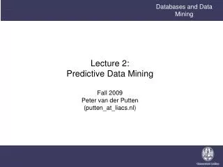
Databases and Data Mining. Lecture 2: Predictive Data Mining Fall 2009 Peter van der Putten (putten_at_liacs.nl). Agenda Today. Recap Lecture 1 Data mining explained Predictive data mining concepts Classification and regression Predictive data mining techniques Logistic Regression

E N D
Databases and Data Mining Lecture 2:Predictive Data MiningFall 2009Peter van der Putten(putten_at_liacs.nl)
Agenda Today • Recap Lecture 1 • Data mining explained • Predictive data mining concepts • Classification and regression • Predictive data mining techniques • Logistic Regression • Nearest Neighbor • Decision Trees • Naive Bayes • Neural Networks • Evaluating predictive models
Sources of (artificial) intelligence • Reasoning versus learning • Learning from data • Patient data • Customer records • Stock prices • Piano music • Criminal mug shots • Websites • Robot perceptions • Etc.
Some working definitions…. • ‘Data Mining’ and ‘Knowledge Discovery in Databases’ (KDD) are used interchangeably • Data mining = • The process of discovery of interesting, meaningful and actionable patterns hidden in large amounts of data • Multidisciplinary field originating from artificial intelligence, pattern recognition, statistics, machine learning, bioinformatics, econometrics, ….
Some working definitions…. • Concepts: kinds of things that can be learned • Aim: intelligible and operational concept description • Example: the relation between patient characteristics and the probability to be diabetic • Instances: the individual, independent examples of a concept • Example: a patient, candidate drug etc. • Attributes: measuring aspects of an instance • Example: age, weight, lab tests, microarray data etc • Pattern or attribute space
Data Preparation • Creating data sets • Feature extraction • Flattening • Longitudinal data set up • … • On attributes • Attribute selection • Attribute construction • … • On attribute values • Outlier removal / clipping • Normalization • Creating dummies • Missing values imputation • ….
Longitudonal set up: predicting into the future • Predictor period • All predictors are measured at end of this period with optional transactional history dating backwards • This point in time corresponds with the ‘current’ situation • No information from ‘future’ (fields nor selections) should be used! • Gestation period • Occurrence of the target behavior doesn’t count in this ‘future’ period • Outcome period • This is the ‘future’ period when behavior is measured Gestation Period Predictor Period Outcome Period
Longitudonal set up: predicting into the future, telco churn example • Predictor period • Snapshot from customer table as of end of April • History of transactions for last month, last three months and last 6 months • Population trimmed down to medium value or higher, near end of contract or out of contract customers • Gestation period • Churn in May or June doesn’t count; we need to predict churn sufficiently in advance • Outcome period • Churn is measured in July Gestation Period Predictor Period Outcome Period
Data mining tasks • Predictive data mining • Classification: classify an instance into a category • Regression: estimate some continuous value • Descriptive data mining • Matching & search: finding instances similar to x • Clustering: discovering groups of similar instances • Association rule extraction: if a & b then c • Summarization: summarizing group descriptions • Link detection: finding relationships • …
Data Mining Tasks: Classification Goal classifier is to seperate classes on the basis of known attributes The classifier can be applied to an instance with unknow class For instance, classes are healthy (circle) and sick (square); attributes are age and weight weight age
Examples of Classification Techniques • Majority class vote • Logistic Regression • Nearest Neighbor • Decision Trees, Decision Stumps • Naive Bayes • Neural Networks • Genetic algorithms • Artificial Immune Systems
Example classification algorithm:Logistic Regression • Linear regression • For regression not classification (outcome numeric, not symbolic class) • Predicted value is linear combination of inputs • Logistic regression • Apply logistic function to linear regression formula • Scales output between 0 and 1 • For binary classification use thresholding
Example classification algorithm:Logistic Regression Classification Linear decision boundaries can be represented well with linear classifiers like logistic regression fe weight fe age
Logistic Regression in attribute space Voorspellen Linear decision boundaries can be represented well with linear classifiers like logistic regression f.e. weight f.e. age
Logistic Regression in attribute space Voorspellen xxxx Non linear decision boundaries cannot be represented well with linear classifiers like logistic regression f.e. weight f.e. age
Logistic Regression in attribute space Non linear decision boundaries cannot be represented well with linear classifiers like logistic regression Well known example: The XOR problem f.e. weight f.e. age
Example classification algorithm:Nearest Neighbour • Data itself is the classification model, so no model abstraction like a tree etc. • For a given instance x, search the k instances that are most similar to x • Classify x as the most occurring class for the k most similar instances
Nearest Neighbor in attribute space Classification = new instance Any decision area possible Condition: enough data available fe weight fe age
Nearest Neighbor in attribute space Voorspellen Any decision area possible Condition: enough data available bvb. weight f.e. age
Example Classification AlgorithmDecision Trees 20000 patients age > 67 yes no 1200 patients 18800 patients Weight > 85kg gender = male? yes no no 400 patients 800 customers etc. Diabetic (%50) Diabetic (%10)
Building Trees:Weather Data example KDNuggets / Witten & Frank, 2000
An internal node is a test on an attribute. A branch represents an outcome of the test, e.g., Color=red. A leaf node represents a class label or class label distribution. At each node, one attribute is chosen to split training examples into distinct classes as much as possible A new case is classified by following a matching path to a leaf node. Building Trees Outlook sunny rain overcast Yes Humidity Windy high normal false true No Yes No Yes KDNuggets / Witten & Frank, 2000
Split on what attribute? • Which is the best attribute to split on? • The one which will result in the smallest tree • Heuristic: choose the attribute that produces best separation of classes (the “purest” nodes) • Popular impurity measure: information • Measured in bits • At a given node, how much more information do you need to classify an instance correctly? • What if at a given node all instances belong to one class? • Strategy • choose attribute that results in greatest information gain KDNuggets / Witten & Frank, 2000
Which attribute to select? • Candidate: outlook attribute • What is the info for the leafs? • info[2,3] = 0.971 bits • Info[4,0] = 0 bits • Info[3,2] = 0.971 bits • Total: take average weighted by nof instances • Info([2,3], [4,0], [3,2]) = 5/14 * 0.971 + 4/14* 0 + 5/14 * 0.971 = 0.693 bits • What was the info before the split? • Info[9,5] = 0.940 bits • What is the gain for a split on outlook? • Gain(outlook) = 0.940 – 0.693 = 0.247 bits Witten & Frank, 2000
Which attribute to select? Gain = 0.247 Gain = 0.152 Gain = 0.048 Gain = 0.029 Witten & Frank, 2000
Continuing to split KDNuggets / Witten & Frank, 2000
The final decision tree • Note: not all leaves need to be pure; sometimes identical instances have different classes Splitting stops when data can’t be split any further KDNuggets / Witten & Frank, 2000
Computing information • Information is measured in bits • When a leaf contains once class only information is 0 (pure) • When the number of instances is the same for all classes information reaches a maximum (impure) • Measure: information value or entropy • Example (log base 2) • Info([2,3,4]) = -2/9 * log(2/9) – 3/9 * log(3/9) – 4/9 * log(4/9) KDNuggets / Witten & Frank, 2000
Decision Trees in Pattern Space Goal classifier is to seperate classes (circle, square) on the basis of attribute age and income Each line corresponds to a split in the tree Decision areas are ‘tiles’ in pattern space weight age
Decision Trees in attribute space Goal classifier is to seperate classes (circle, square) on the basis of attribute age and weight Each line corresponds to a split in the tree Decision areas are ‘tiles’ in attribute space weight age
Example classification algorithm:Naive Bayes • Naive Bayes = Probabilistic Classifier based on Bayes Rule • Will produce probability for each target / outcome class • ‘Naive’ because it assumes independence between attributes (uncorrelated)
Bayes’s rule • Probability of event H given evidence E : • A priori probability of H : • Probability of event before evidence is seen • A posteriori probability of H : • Probability of event after evidence is seen from Bayes “Essay towards solving a problem in the doctrine of chances” (1763) Thomas Bayes Born: 1702 in London, EnglandDied: 1761 in Tunbridge Wells, Kent, England KDNuggets / Witten & Frank, 2000
Naïve Bayes for classification • Classification learning: what’s the probability of the class given an instance? • Evidence E = instance • Event H = class value for instance • Naïve assumption: evidence splits into parts (i.e. attributes) that are independent KDNuggets / Witten & Frank, 2000
Weather data example Evidence E Probability of class “yes” KDNuggets / Witten & Frank, 2000
Probabilities for weather data KDNuggets / Witten & Frank, 2000
Probabilities for weather data • A new day: KDNuggets / Witten & Frank, 2000
Extensions • Numeric attributes • Fit a normal distribution to calculate probabilites • What if an attribute value doesn’t occur with every class value?(e.g. “Humidity = high” for class “yes”) • Probability will be zero! • A posteriori probability will also be zero!(No matter how likely the other values are!) • Remedy: add 1 to the count for every attribute value-class combination (Laplace estimator) • Result: probabilities will never be zero!(also: stabilizes probability estimates) witten&eibe
Naïve Bayes: discussion • Naïve Bayes works surprisingly well (even if independence assumption is clearly violated) • Why? Because classification doesn’t require accurate probability estimates as long as maximum probability is assigned to correct class • However: adding too many redundant attributes will cause problems (e.g. identical attributes) witten&eibe
Naive Bayes in attribute space Classification NB can model non fe weight fe age
Example classification algorithm:Neural Networks • Inspired by neuronal computation in the brain (McCullough & Pitts 1943 (!)) • Input (attributes) is coded as activation on the input layer neurons, activation feeds forward through network of weighted links between neurons and causes activations on the output neurons (for instance diabetic yes/no) • Algorithm learns to find optimal weight using the training instances and a general learning rule.
Neural Networks • Example simple network (2 layers) • Probability of being diabetic = f (age * weightage + body mass index * weightbody mass index) age body_mass_index Weightbody mass index weightage Probability of being diabetic
Neural Networks in Pattern Space Classification Simpel network: only a line available (why?) to seperate classes Multilayer network: Any classification boundary possible f.e. weight f.e. age
Evaluating Classifiers • Error measures • Basic classification evaluation measure: Accuracy = 78% on test set 78% of classifications were correct • Root mean squared error (rmse - regression), Area Under the ROC Curve (AUC), confusion matrices • Hold out validation, n fold cross validation, leave one out validation • Build a model on a training set, evaluate on test set • Hold out: single test set (f.e. one thirds of data) • n fold cross validation • Divide into n groups • Perform n cycles, each cycle with different fold as test set • Leave one out • Test set of one instance, cycle trough all instances
Evaluating Classifiers • Investigating the sources of error: bias variance decomposition • Informal definition • Intrinsic error: error of the (hypothetical) optimal classifier • Bias: error due to limitations of model representation (eg linear classifier on non linear problem); even with infinite data there will be bias • Language bias • Search bias • Overfitting avoidance bias • Variance: error due to instability of classifier over different samples; error due to sample sizes, overfitting
Example ResultsPredicting Survival for Head & Neck Cancer TNM Symbolic TNM Numeric Average and standard deviation (SD) on the classification accuracy for all classifiers
Example Results Head and Neck Cancer:Bias Variance Decomposition • What is the largest error component? • What component is most important in explaining the difference across models?