Pro Forma Analysis
Pro Forma Analysis. Agribusiness Finance LESE 306 Fall 2009. PRESENT. PAST. FUTURE. Historical analysis Comparative analysis Historical price and yield trends. Pro forma analysis Forming expectations about future prices, costs and productivity Ad hoc extrapolations


Pro Forma Analysis
E N D
Presentation Transcript
Pro Forma Analysis Agribusiness FinanceLESE 306 Fall 2009
PRESENT PAST FUTURE • Historical analysis • Comparative analysis • Historical price and yield trends • Pro forma analysis • Forming expectations about future prices, costs and productivity • Ad hoc extrapolations • Projections based upon available outlook data • Projections based upon econometric analysis
Timeline Required for Capital Budgeting… Assume it is the year 2009 and John Deere wants to project farm machinery and equipment sales over the next six years to determine if plant expansion is necessary. 2009 2010 2011 2012 2013 2014 2015
Timeline Required for Capital Budgeting… Assume it is the year 2009 and John Deere wants to project farm machinery and equipment sales over the next six years to determine if plant expansion is necessary. 2009 2010 2011 2012 2013 2014 2015 Capital budgeting models of investment decisions require projections of the annual revenue and cost values over the entire 2010 to 2015 time period. Page 89 in booklet
Remember the definition of annual net cash flows Page 74 in booklet
Must project Annual yield Must project Annual price Page 85 in booklet
Ad Hoc Modeling Approaches • Naïve model – using last year’s prices, costs and yields • Simple linear trend extrapolation of historical prices, costs and yields • Moving Olympic average • Using assumptions made by others
Ad Hoc Modeling Approaches Naïve model: Pt = Pt-1 Linear trend: Pt = a0 + a1(Year) Olympic average: Pt = Last 5 year annual price, dropping high and low and calculate the average of the remaining three year’s price.
Econometric Model Approach • Capturing future supply/demand impacts on prices and unit costs • Linkages to commodity policy • Linkages to domestic economy • Linkages to the global economy
Concept of Derived Demand for Farm Machinery The demand for farm machinery is driven by the expected net economic benefit from use of the machine….
D D S S Crop Market Equilibrium Price S D • Supply consists of: • Beginning stocks • Production • Imports Pe • Demand consists of: • Industrial use • Feed use • Exports • Ending stocks Quantity Qe Page 45 in booklet
Forecasting Future Commodity Price Trends D $7 S D = a – bP + cYD + eX $4 Own price Other factors Disposable income $1 10 Page 45 in booklet
Forecasting Future Commodity Price Trends D $7 S Own price Input costs Other factors $4 S = n + mP – rC + sZ $1 10 Page 46 in booklet
Projecting Commodity Price D $7 S D = 10 – 6P + .3YD + 1.2X D = S $4 S = 2 + 4P – .2C + 1.02Z $1 10 Substitute the demand and supply equations into the the equilibrium condition and solve for price Page 46 in booklet
The Market Model Demand equations: Qd,i = a0 - a1(Price) + ai (demand shifters) Supply equation: Qs,i = b0 +b1(price) + bi (supply shifters) Market equilibrium: ΣQd,i = ΣQs,i
Econometric Analysis Based on Time Trend Extrapolation It = f(Yeart)
A linear time trend projection of future farm machinery and equipment sales therefore does a poor job of predicting future sales activity.
Econometric Analysis Based on Investment Theory It = f{[E(Pt)×E(Qt)]/E(ct)} Incorporates the economic concepts of MVP and MIC
An econometric model based on investment theory does a muchbetter job of predicting future sales activity.
Econometric Analysis – Food Use Own price elasticity Income elasticity Cross price elasticity
Observed and Predicted Values For Wheat Food Use
Remaining Steps to Forecasting the Price of Commodity • Develop similar econometric equations for the other uses of wheat (feed use, exports and ending stock). • Develop econometric equations for production and import supply. • Substitute the estimated equations into the market equilibrium definition (QD=QS) and solve for the price whereexcess demand equals zero.
Point Forecast Assumptions Assumes perfect knowledge of outcomes in all 5 areas!!!! PE QE Page 47 in booklet
Structural Pro Forma Analysis Supply-side risk for a given price… PE Page 47 in booklet QLQEQH
Structural Pro Forma Analysis Demand and supply-side risk and potential price variability… PH PE PL QLQEQH Page 47 in booklet
A 48 percent chance that the price of wheat will be less than $4.16 Page 85 in booklet
Potential Variability in Wheat Price 2008/09 MY Given Historical Variability in Growing Conditions Ratings Page 96 in booklet
$2.50 $3.00 $3.50 Triangular Probability Distribution Page 131 in booklet
Conclusions • Econometric models preferred over naïve models and linear time trend models. • Much more accurate. • Provide much more information (e.g., elasticities). • Allow for sensitivity analysis with independent (exogenous) variables when evaluating potential variability about expected trends.
G is the expected rate of appreciation Page 82 in booklet
Allowing for unequal annual net cash flows…. Page 79 in booklet
Allowing for unequal discount rates… Page 63 in booklet
Adjusting Discount Rate • We said to date that the discount rate is the firm’s opportunity rate of return. • Realistically we must allow for business risk by including a risk premium. • Realistically we must also allow for financial risk by adding an additional risk premium.
Business Risk • Risk associated with price of the product or products you are producing. • Risk associated with the unit costs for the inputs used in producing the product(s). • Risk associated with yields (productivity) in production. • NCFi=Piyieldsiunit sales – Ciunit inputs
Accounting for Business Risk RRRH,i RRRL,i RFREE,i .05 RFREE,i = risk free rate of return (i.e., govt. bond rate) RRRL,i = required rate of return for lowly risk averse RRRH,i = required rate of return for highly risk averse Page 132 in booklet
Increasing Risk Over Time Probability Product price distribution E(P) Year 1 Year 1 Year 10 Year 10 $2.95 $3.05 $3.15 Pessimistic price Expected price Optimistic price