Download

1 / 38
380 likes | 409 Vues
Discover all frequent closed patterns in datasets with a user-defined support threshold using CARPENTER algorithm. Learn about row enumeration strategy, features, and algorithms like COBBLER. Prune methods and performance comparisons included.

E N D
Frequent Closed Pattern Search By Row and Feature Enumeration
Outline • Problem Definition • Related Work: Feature Enumeration Algorithms • CARPENTER: Row Enumeration Algorithm • COBBLER: Combined Enumeration Algorithm
Problem Definition • Frequent Closed Pattern:1) frequent pattern: has support value higher than the threshold2) closed pattern: there exists no superset which has the same support value • Problem Definition:Given a dataset D which contains records consist of features, our problem is to discover all frequent closed patterns respect to a user defined support threshold.
Related Work • Searching Strategy:breadth-first & depth-first search • Data Format:horizontal format & vertical format • Data Compression Method: diffset, fp-tree, etc.
Typical Algorithms • CLOSET • feature enumeration • horizontal format • depth-first search • fp-tree technique • APRIORI • feature enumeration • horizontal format • breadth-first search • CHARM • feature enumeration • vertical format • depth-first search • deffset technique
CARPENTER CARPENTER stands for Closed Pattern Discovery by Transposing Tables that are Extremely Long • Motivation • Algorithm • Prune Method • Experiment
Motivation • Bioinformatic datasets typically contain large number of features with small number of rows. • Running time of most of the previous algorithms will increase exponentially with the average length of the transactions. • CARPENTER’s search space is much smaller than that of the previous algorithms on these kind of datasets and therefore has a better performance.
Algorithm • The main idea of CARPENTER is to mine the dataset row-wise. • 2 steps: • First, transpose the dataset • Second , search in the row enumeration tree.
Transpose Table • Feature a, b, c, d. • Row r1, r2 , r3, r4. transpose project on (r2 r3) original table transposed table projected table
Row Enumeration Tree r1r2r3r4 { } r1 r2 r3 {bc} r1 r2 {bc} • According to the transposed table, we build the row enumeration tree which enumerates row ids with a pre-defined order. • We do a depth first search in the row enumeration tree with out any prune strategies. r1 r2 r4 {} r1 r3 {bc} r1 r3 r4 { } minsup=2 bc: r1r2r3 bcd: r2r3 d: r2r3r4 r1 {abc} r1 r4 {} r2 r3 {bcd} r2 r3 r4 {d } { } r2 {bcd} r2 r4 {d} r3 r4 {d } r3 {bcd} r4 {d}
Prune Method 1 • In the enumeration tree, the depth of a node is the corresponding support value. • Prune a branch if there won’t be enough depth in that branch, which means the support of patterns found in the branch will not exceed the minimum support. minsup 4 r2 r3 {bcd} r2 {bcd} r2 r4 {d} depth= 1 sup =1 2 sub-nodes Max support value in branch “r2” will be 3, therefore prune this branch.
Prune Method 2 • If rj has 100% support in projects table of ri, prune the branch of rj. r2 {bcd} r2 r3 {bcd} r2 r3 r4 {d} r2 r4 {d} r2 r3 {bcd} r2 r3 r4 {d} r3 has 100% support in the projected table of “r2”, therefore branch “r2 r3” will be pruned and whole branch is reconstructed.
Prune Method 3 • At any node in the enumeration tree, if the corresponding itemset of the node has been found before, we prune the branch rooted at this node. r2 {bcd} r2 r3 {bcd} r2 r4 {d} r3 {bcd} r3 r4 {d} Since itemset {bcd} has been found before, the branch rooted at “r3” will be pruned.
Performance • We compare 3 algorithms, CARPENTER, CHARM and CLOSET. • Dataset (Lung Cancer) has 181 rows with 12533 features. • We set 3 parameters, minsup, Length Ratio and Row Ratio.
minsup Lung Cancer, 181 rows, length ratio 0.6,row ratio 1. Running time of CARNPENTER changes from 3 to 14 second
Length Ratio Lung Cancer, 181 rows, sup 7 (4%), row ratio 1 Running time of CARPENTER changes from 3 to 33 seconds
Row Ratio Lung Cancer, 181 rows, length ratio 0.6,sup 7 (4%) Running time of CARPENTER changes from 9 to 178 seconds
Conclusion • We propose an algorithm call CARPENTER for finding closed pattern on long biological datasets. • CARPENTER perform row enumeration instead of column enumeration since the number of rows in such datasets are significantly smaller than the number of features. • Performance studies show that CARPENTER is much more efficient in finding closed patterns compared to existing feature enumeration algorithms.
COBBLER • Motivation • Algorithm • Performance
Motivation • With the development of CARPENTER, existing algorithms can be separated into two parts. • Feature enumeration: CHARM, CLOSET, etc. • Row enumeration: CARPENTER • We have two motivations to combine these two enumeration methods
Motivation 1. We can see that these two enumeration methods have their own advantages on different type of data set. Given a dataset, the characteristic of its sub-dataset may change. sub-dataset dataset project more features than rows more rows than features 2. Given a dataset with both large number of rows and features, a single row enumeration algorithm or a single feature enumeration method can not handle the dataset.
Algorithm • There are two main points in the COBBLER algorithm • How to build an enumeration tree for COBBLER. • How to decide when the algorithm should switch from one enumeration to another. • Therefore, we will introduce the idea of dynamic enumeration tree and switching condition
Dynamic Enumeration Tree • We call the new kind of enumeration tree used in COBBLER the dynamic enumeration tree. • In dynamic enumeration tree, different sub-tree may use different enumeration method. original transposed We use the table as an example in later discussion
Single Enumeration Tree abcd { } r1r2r3r4 { } r1r2r3 {c} abc {r1} ab {r1} r1r2 {ac} r1r2r4 { } abd { } ac {r1r2} acd { r2} r1r3 {bc} r1r3r4 { } a {r1r2} r1 {abc} ad {r2} r1r4 { } r2r3r4 { } bc {r1r3} bcd { } r2r3 {c} { } b {r1r3} { } r2 {acd} bd { } r2r4 {d } cd {r2 } c {r1r2r3} r3r4 { } r3 {bc} d {r2r4} Feature enumeration Row enumeration r4 {d}
Dynamic Enumeration Tree abcd { } abc {r1} r1r2 {c} ab {r1} r1 {bc} abd { } a {r1r2} ac {r1r2} acd { r2} r2 {cd} a {r1r2} ad {r2} r1 {c} r1r3 { c} { } b {r1r3} r3 { c} abc: {r1} ac: {r1r2} acd: {r2} c {r1r2r3} r2 {d } d {r2r4} Feature enumeration to Row enumeration
Dynamic Enumeration Tree r1r2r3r4 { } r1r2r3 {c} ab {} r1r2 {ac} a {r2} r1r2r4 { } ac { r2} r1r3 {bc} r1r3r4 { } b {r3} bc {r3 } r1 {abc} r1 {abc} r1r4 { } c {r2r3 } ac {r1 } acd { } a {r1} ad { } { } r2 {acd} cd { } ac: {r1r2} bc: {r1r3} c: {r1r2r3} c {r1r3} d {r4 } bc {r1 } b {r1 } r3 {bc} c {r1r2 } r4 {d} Row enumeration to Feature Enumeration
Dynamic Enumeration Tree • When we use different condition to decide the switching, the structure of the dynamic enumeration tree will change. • No matter how it switches, the result set of closed pattern will be the same as the result of the single enumeration .
Switching Condition • The main idea of the switching condition is to estimate the processing time of the a enumeration sub-tree, i.e., row enumeration sub-tree or feature enumeration sub-tree. • Define some characters.
Switching Condition • Suppose r=10, S(f1)=0.8, S(f2)=0.5, S(f3)=0.5, S(f4)=0.3 and minsup=2 • Then the estimated deepest node under f1 is f1f2f3, since • S(f1)*S(f2)*S(f3)*r=2 >minsup • S(f1)*S(f2)*S(f3)*S(f4)*r=0.6 < minsup
Experiments • We compare 3 algorithms, COBBLER, CHARM and CLOSET+. • One real-life dataset and one synthetic data. • We set 3 parameters, minsup, Length Ratio and Row Ratio.
minsup Synthetic data Real-life data (thrombin)
Length and Row ratio Synthetic data
Discussion • The combination of row and feature enumeration also makes some disadvantage • The cost to calculate the switching condition and the cost of bad decision. • The increased cost in pruning, maintain two set of pruning system.
Discussion • We may use other more complicated data structure in our algorithm to improve the performance, e.g., the vertical data format and diffset technique. • And more efficient switching condition may improve the algorithm further.
Conclusion • The COBBLER algorithm gives better performance on dataset where the advantage of switching can be shown, e.g., complex dataset or dataset has both large number of rows and features. • For simple characteristic data, a single enumeration algorithm may be better.
Future Work • Using other data structure and technique in the algorithm. • Extend COBBLER to handle dataset that can not be fitted into memory.