Values from Table
Values from Table. m -3. Other values …. Thermal admittance of dry soil ~ 10 2 J m -2 s -1/2 K -1 Thermal admittance of wet saturated soil ~ 10 3 J m -2 s -1/2 K -1. Soil density, thermal conductivity, thermal admittance. Elevated % of quartz and clay minerals. Water content.
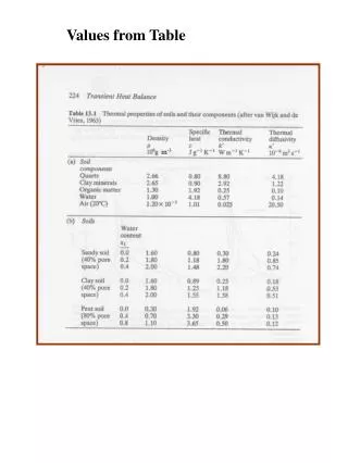

Values from Table
E N D
Presentation Transcript
Other values…. Thermal admittance of dry soil ~ 102 J m-2 s-1/2 K-1 Thermal admittance of wet saturated soil ~ 103 J m-2 s-1/2 K-1
Soil density, thermal conductivity, thermal admittance. Elevated % of quartz and clay minerals Water content High values Sandy Clay Peat Low values Elevated % of organic matter (this is only qualitative the relations are non linear)
Amplitude of the temperature wave at the surface DT. Elevated % of quartz and clay minerals Water content Low values Sandy Clay Peat High values Elevated % of organic matter (this is only qualitative the relations are non linear)
Specific heat Elevated % of quartz and clay minerals Water content Low values Sandy Clay Peat High values Elevated % of organic matter (this is only qualitative the relations are non linear)
Thermal diffusivity. Elevated % of quartz and clay minerals Water content High values Sandy Clay Peat Low values Low values Elevated % of organic matter (this is only qualitative the relations are non linear)
Examples: Dry Sandy Soil (40% pore space)
Limitations of the previous approach: • Measurements show that the ground heat flux is not sinusoidal in time. In particular during night-time is more uniform and much flatter. • The assumed sinusoidal variation of the surface temperature may be not realistic. • The simplifying assumption of the homogeneity of the submedium is often not realized. max min 9 hrs
1st approach:Statistical parameterizations Reasonable expectation that QG is a fraction of Q* forcing. The surface QG leads the Q* forcing by about 3 hours. Therefore a daily plot of QG vs Q* results in a hysteresis loop
This loop can be modeled as Where a, b, c are deduced from measurements. Ex. For bare soil (Novak, 1981): a=0.38,b=0.56 hrs, and c=-27.3 W m-2 This approach ignores the role of wind (Convection) in heat sharing at the surface
2nd approach: physically based models They take into account net radiation, latent and sensible heat fluxes at the surface The Force-Restore method (Deardorff, 1978) Two layer approximation A shallow thermally active layer near the surface, and a thicker layer below.
Energy budget of the shallow layer Q*=net radiation QE=Latent Heat Flux QH=Sensible Heat Flux QG=Ground Heat Flux TG=ground temperature of the shallow layer d= depth of the shallow layer C= specific heat r=soil density N.B. Non radiative positive fluxes are directed away from the surface. QH and QE are positive when upward, QG when downward. Q*(radiative flux) is positive when downward.
rc=Cs is the heat capacity of the soil, function of the water content. Dz
To estimate Tm two possibilities: • Constant (equal to the mean air temperature of the previous 24hrs) • Computed assuming that the ground heat flux at the bottom of the thicker layer is zero. Restoring term Surface forcing term If the surface forcing term is removed, the restoring term will cause TG to move exponentially towards Tm
Multi-Layer Soil Models (Tremback and Kessler, 1985) Compute the soil temperature in several layers in the soil solving numerically: The thermal diffusivity k is computed as a function of the soil heat capacity and soil moisture potential
The forces which bind soil water are related to the soil porosity and the soil water content (S, volume of water per volume of soil). The forces are weakest for open textured, wet soils and greatest for a clay soil
For a given soil, the potential increases as S decreases. It is relatively easy to extract moisture from a wet soil but as it dries out it becomes increasingly difficult to remove additional units
Vertical flux of liquid water in soil (in absence of percolating rain) is result of: • Gravity • Vertical water potential gradient (flux gradient relationship as for heat). Darcy’s Law g The effect of evapotranspiration is to create a vertical positive potential gradient which becomes greater than the opposing gravitational gradient and encourage the upward movement of water.
Soil heat flux measurements (Oke, 374-5) In theory QG can be calculated from TG profiles and knowledge of k or k – in practice this is not really possible, since the values of k and k are variable and very difficult to measure. Most use soil heat flux plats (similar idea to net radiometer thermopile) Plates should be inserted in un-disturbed soil (few cm depth), and not right at the surface. The depth depends on the nature of the soil and the presence of roots. Need to consider energy budget between plate and surface
z Plate measured measured Soil heat capacity estimated from volume fraction of mineral, organic matters and water CS =Cm qm + Co qo + Cw qw + Ca qa