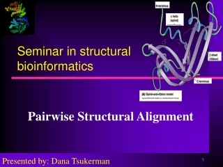
Seminar in structural bioinformatics
650 likes | 680 Vues
Learn about structural alignment vs. sequence alignment, algorithm implementation, and 3-D transformation in this seminar. Understand how structural alignment helps in protein structure comparison and drug design.

Seminar in structural bioinformatics
E N D
Presentation Transcript
Seminar in structural bioinformatics Pairwise Structural Alignment Presented by: Dana Tsukerman
Outline • Definitions. • What is structural alignment? • Why structural alignment? structural alignment vs. sequence alignment • Problem definition • Background preparing the ground for the algorithm. • The algorithm
Outline - cont. • Implementation of the algorithm and an example of using a real software, based on the algorithm that will be presented. • Method results. • Method discussion • Method summary. • Extensions and additional features - a look ahead. • Lecture summary.
Definitions • Sequence alignment (remainder from last lecture), unambiguously distinguishes only between protein pairs of similar structure and non-similar structures when the pairwise sequence identity is high. • Structure alignment - the precise arrangement of the amino acid side chains in the three dimensional structure of the protein that dictates its function.
Quick rehearsal - Basic terms • Primary structure refers to the order (and sequence) of amino acids along one chain. • Some regions form regular local structure (folding patterns): • Alpha helices • Beta strands • Collectively called secondary structure elements (SSEs). • Regions connecting SSEs areloops. • Secondary structure is the description of the type and locations of the SSEs. • Tertiary structure is the 3-D coordinates of the atoms in a chain. • Quaternary structure describes the spatial packing of several folded chains (not all proteins have a quaternary structure).
Quick rehearsal - Basic terms regular hydrogen bond patterns of backbone atoms
Turn or coil Alpha-helix Beta-sheet Loop and Turn 3D observation of proteins
3D observation of proteins “If one looks at the collection of protein structures, one is reminded of the works of an Origami artist: Certain basic folding patterns are used over and over again and cleverly modified by minor adaptations to generate a wide variety of different protein structures. Where one such folding units is insufficient to generate the required complexity, multiple domains can be combined, such as in the camel or giraffe structure on this picture.”
Comparison in 3D • Starting from an example: A B A B C C E D D E back
Comparison in 3D • Rotation and translation coordinates - 6 degrees of freedom. • The method is independentof the amino acid sequence. What does it mean? This method is insensitive to insertions, deletions and displacements of equivalents substructures betweens the molecules being compared. • Proteins with similar sequences adopt very similar structures.
Why 3D comparison? Wait a minute - isn’t sequence comparison enough?
Why 3D comparison? • Structures are more conserved than sequences. • Detection of distant evolutionary relationships. • Structural alignment can imply a functional similarity that isn’t detectable from a sequence alignment. • The protein docking problem. • Structure based drug design. • Applications and implications to the protein folding problem.
Why 3D comparison? Cont. • For homologous proteins, this provides the “gold standard” for sequence alignment. • For nonhomologous proteins, it allows us to identify common substructures of interest. • Allows us to classify proteins into clusters, based on structural similarity. • Design and engineering of synthetic proteins.
Problem Definition • Input: 3-D coordinate data of the structures to be compared. • Output: regions of structural similarity (more than one, if exists), that lead to the “best” alignment. • NP-Hard. Most atoms matched with the lowest RMSD What’s “best”?
Our goal Find out the correspondence between the structures transformation T
Preparing the ground • Transformation: definition. • How can we evaluate the match we found? RMSD: rehearsal from the opening lecture. • Other methods besides the one we will discuss: and why our method is better. • Progression rule: definition. • PDB: functionality rehearsal. • Geometric Hashing: introduction.
3-D Transformation • Rotation - the movement of a body in such a way that any given point of that body remains at a constant distance from some other fixed point. Will be denoted by R. • Translation - the transformation of moving every point by a fixed distance in the same direction (addition of a constant vector to every point). Will be denoted by T. • What is preserved under translation and rotation? relative distances within an object (e.g. Shapes) • In total, the 3-D transformation has 6 degrees of freedom: 3 for rotation and 3 for translation.
RMSD - rehearsal • A tool we use to evaluate the correspondence we found. • RMSD - Root Mean Square Deviation Where, • n = number of atoms • x, y = the proteins we want to compare (structures) • We want to find 3-D transformation T*, such that the RMSD will be minimal, i.e.: • We know how to do that in O(n).
Other methods for structural alignment • Dynamic programming - building a score matrix, with a score for each pair of residues. or • Other improvements of that method. • Simplify the problem by moving from 3D space to 2D space sacrificing the optimum result for the speed. • Comparing secondary structure elements (SSE) • Our method allows access to problems that couldn’t be approached previously by sequence-order-dependent structural comparison methods, like the docking problem.
Progression rule • Rule definition: for elements i and k from one sequence and elements j and l from the other sequence, if element i is matched to element j and element k is matched to element l, and if k is to the right of i in the first sequence, the l must also be to the right of j in the second sequence. • For example, the structures we saw at the beginning couldn’t be found similar by a progression rule based method (sequence -dependent). Example
PDB - Protein Data Bankhttp://www.rcsb.org/pdb/index.html • International structure database. • Archive of experimentally determined 3-D structures of biological macromolecules, together with extensive annotation. • Established at Brookhaven National Laboratories in 1971. in the beginning it held 7 structures. • In 2003, 4,831 structures were deposited to the PDB archive. • January 2004 snapshot: 23,792 released atomic coordinate entries.
Geometric hashing • Introduced for model-based object recognition in computer vision. • Goal: identify and locate in an image all the instances of models which appear in the system’s database. • Represents the objects to be compared in a translational and rotational invariant fashion. • On which the first step of the algorithm presented today is based.
Geometric hashing - cont. • We search for a way to represent object in a way we will be able to move them, and the representation won’t change. HOW? Building triangles! for nodes: triangles! The triangle’s sides length doesn’t change when we move it or rotate it, and thus invariant!
now please pay attention… Wake Up!
The algorithm – major steps • Find (relatively small) subsets of the structures that form an initial match; • Find clusters in initial matches that represent similar transformations; • Extend the clusters to contain additional matching pairs of residues.
Motivation remainder now let's jump into the water...
Step 1 - Finding seed matches • Goal: search through the structures to find candidate initial matches. • Those will be referred as seed matches. • Most difficult and time consuming step. • Extensive search of the structures. • How to represent? • Remember what we talked about in geometric hashing?
Finding seed matches - cont. • Seedmatch - list of matching pairs of atoms. • Pair - correspondence between atoms from different structures. • Assumption: the structures to be compared are described by sets of interest points and their 3-D coordinates (for example: Cα atoms). • Model & Target.
Finding seed matches - cont. • Redefinition of the problem: is there a rotated and translated subset of the interest points of the target which matches those of the model? • Two phases: • preprocessing • recognition
Preprocessing - intro. • Goal: represent the information about the atoms of the model molecule in a rotation and translation invariant manner. • Off-line. Why? • This information will be later used in the recognition phase. • 3 non-collinear atoms specify a unique orthonormal reference frame (unique coordinate system). This will be a full reference frame.
b a c Preprocessing - intro. • We won’t use a full reference frame: only 2 atoms (not unique). Those 2 atoms will be called reference set. • Each atom b in the molecule is represented by the triplet of distances of the sides of the triangle formed between b and the atoms of the reference set. Reference set: (c,a)
Reference frames - clarification Note: the example is in the 2-D case (basic ideas the same as the 3-D case) Same shape, different reference frames
How to store the information efficiently? Preprocessing
Preprocessing • Hash table: representation of each model atom triplets of distances (from the atom to reference pair) the corresponding reference pair and the atom which obtained this key. • Note: • each atom has a redundant representation in all possible reference sets. • Many triangles can occupy the same hash table entry.
Preprocessing Complexity Discussion • The complexity is highly dependent on the invariants we use for hashing. • Complexity: O(n3) • n is the # of atoms in the model. But…We can do better! we will later see an optimization that will reduce the complexity to O(n2).
Preprocessing example Note: the example is in the 2-D case (basic ideas the same as the 3-D case) • Reference frame here is a pair of coordinates. • For instance, in cell (3, 2) we find point #2, in both reference frames, and so we store those reference frames in the hash table H(3, 2).
Recognition - intro. • Goal: discover candidate matching substructures in the target and model molecules. • Referenceset - pair of atoms. • Each such matching substructure is based on a certain reference set, which appears both in the model and target molecules.
Recognition algorithm • For each reference set of the target: • Hold a votecounter for each reference set appearing in the hash table. • any ideas what will it hold? • Of course, it will hold the current number of matching atoms, and the list of matching pairs. • We will call this list the vote list. • In the beginning: the list is initialized with null. • Pick a target atom (take predefined threshold distance into consideration).
Recognition - cont. • Use the 3 sides of the triangle formed to compute their hash table key. • Access the hash table in this key • Extract all the model triangles in this entry. • For each triangle: • Vote_counter++; • Vote_list.add(current_triangle); • Go back to picking another atom, until we considered all of them.
Recognition - cont. • Check the vote counters of all the entries and consider the ones with a large # of votes. • Verification. • Choose another reference set in the target molecule and go back to the beginning. • Complexity: O(n3*k) • k indicates the # of triangles in each hash table entry. • Can be of order O(n2) after optimizing preprocessing.
Recognition example Note: the example is in the 2-D case (basic ideas the same as the 3-D case) For instance, let’s look on point #f, it’s coordinates are (0, 4) and so this is the key to H. H(0,4) contains the reference frame (1,3), thus it’s counter will be increased (a vote for the base pairs in H) and the pair (7, f) will be added to the matched list. Why (7, f)?
Step 2 - Clustering • Goal: clustering the seed matches that represent almost identical transformations. • Why clustering? Many of the seed matches obtained in step 1 represent the same transformation (but contain different pairs of matching atoms). • We use the lists of matching atoms to compute the 3-D rotation and translation, which gives us the minimal least squares distance between the target and the model.
Clustering - cont. • The computed 3-D transformation has 6 parameters (3 for rotation (angles) and 3 for translation (distances)). • Join similar transformations into new groups. • What's similar? • Small 6-D distance between the parameter vectors of the transformations. • Clustering algorithm (iterative): • At the beginning, each seed match forms a group represented by 6 parameters of it’s transformation.
Clustering - cont. • The pair of groups having the minimal distance between their transformations is chosen and a new group is formed by merging these two groups. • Who will be the parameters of the new group? • A threshold is defined to determine an end to the algorithm. • What do we have so far? • # of groups, each represents one transformation obtained by averaging the individual transformations that were joined to the group.
Clustering - cont. • The seed match of a group is obtained by choosing matching pairs from the original seed matches that composed the group. • But, we don’t take the union of all pairs! • Improve accuracy by choosing pairs that appear in at least certain percentage of the seed matches. • The new correspondence lists are considered more reliable than in step 1. • Complexity: m = # of seed matches to be clustered.
Step 3 - Extending • Goal: extend the correspondence lists from step 2 to contain additional matching pairs. • Remember! the transformation representing each group was computed by taking the average of the initial transformation. • How can we find more matches? • Compute again a transformation which gives the minimal least squares distance between the matched pairs. • The pairs that survive the second transformation are candidate additional matches.
Extending - intro. • :# of iterations to extend each seed match (small constant). • ε - maximum allowed distance. • At iteration i we extend the match to contain pairs of atoms that lie at a maximum distance of
Extending - algorithm • For iteration i: • Find the transformation of the current match using least squares procedure. • Transform the target according to this transformation. • Remove pairs from the current match that lie in a distance larger than • Extend the match by heuristic matching algorithm (given a threshold value).