Data Flow Analysis 1 15-411 Compiler Design
440 likes | 467 Vues
Explore the concepts of abstract syntax trees (AST) and control flow graphs (CFG) in compiler design. Learn about data flow analysis and its applications in optimizing program code.

Data Flow Analysis 1 15-411 Compiler Design
E N D
Presentation Transcript
Data Flow Analysis 115-411 Compiler Design These slides live on the Web. I obtained them from Jeff Foster and he said that he obtained them from Alex Aiken October 5, 2004
Compiler Structure Abstract Syntax tree Control Flow Graph • Source code parsed to produce abstract syntax tree. • Abstract syntax tree transformed to control flow graph. • Data flow analysis operates on the control flow graph (and other intermediate representations). Source code Object code
Abstract Syntax Tree (AST) • Programs are written in text • as sequences of characters • may be awkward to work with. • First step: Convert to structured representation. • Use lexer (like lex) to recognize tokens • Use parser (like yacc) to group tokens structurally • often produce to produce AST
Abstract Syntax Tree Example • x := a + b; • y := a * b • While (y > a){ • a := a +1; • x := a + b • } program while … = x + > block … a b = y a + a a 1
ASTs • ASTs are abstract • don’t contain all information in the program • e.g., spacing, comments, brackets, parenthesis. • Any ambiguity has been resolved • e.g., a + b + c produces the same AST as (a +b) + c.
Disadvantages of ASTs • ASTs have many similar forms • e.g., for while, repeat , until, etc • e.g., if, ?, switch • Expressions in AST may be complex, nested • (42 * y) + ( z > 5 ? 12 * z : z +20) • Want simpler representation for analysis • … at least for dataflow analysis.
Control-Flow Graph (CFG) • A directed graph where • Each node represents a statement • Edges represent control flow • Statements may be • Assignments x = y op z or x = op z • Copy statements x = y • Branches goto L or if relop y goto L • etc
Control-flow Graph Example • x := a + b; • y := a * b • While (y > a){ • a := a +1; • x := a + b • }
Variations on CFGs • Usually don’t include declarations (e.g. int x;). • May want a unique entry and exit point. • May group statements into basic blocks. • A basic block is a sequence of instructions with no branches into or out of the block.
Control-Flow Graph with Basic Blocks • X := a + b; • Y := a * b • While (y > a){ • a := a +1; • x := a + b • } • Can lead to more efficient implementations • But more complicated to explain so… • We will use single-statement blocks in lecture
CFG vs. AST • CFGs are much simpler than ASTs • Fewer forms, less redundancy, only simple expressions • But, ASTs are a more faithful representation • CFGs introduce temporaries • Lose block structure of program • So for AST, • Easier to report error + other messages • Easier to explain to programmer • Easier to unparse to produce readable code
Data Flow Analysis • A framework for proving facts about program • Reasons about lots of little facts • Little or no interaction between facts • Works best on properties about how program computes • Based on all paths through program • including infeasible paths
Available Expressions • An expression e = x op y is available at a program point p, if • on every path from the entry node of the graph to node p, e is computed at least once, and • And there are no definitions of x or y since the most recent occurance of e on the path • Optimization • If an expression is available, it need not be recomputed • At least, if it is in a register somewhere
Data Flow Facts • Is expression e available? • Facts: • a + b is available • a * b is available • a + 1 is available
Gen and Kill statement on the set of facts? • What is the effect of each stmt gen kill a + b x = a + b a * b y = a * b a + b a * b a = a + 1 a + 1
∅ {a + b} {a + b, a * b} {a + b} {a + b} {a + b, a * b} {a + b} Ø {a + b} Computing Available Expressions
Terminology • A join point is a program point where two branches meet • Available expressions is a forward, mustproblem • Forward = Data Flow from in to out • Must = At joint point, property must hold on all paths that are joined.
Data Flow Equations • Let s be a statement • succ(s) = {immediate successor statements of s} • Pred(s) = {immediate predecessor statements of s} • In(s) program point just before executing s • Out(s) = program point just after executing s • In(s) = Is’ 2 pred(s) Out(s’) • Out(s) = Gen(s) [ (In(s) – Kill(s)) • Note these are also called transfer functions
Liveness Analysis • A variable v is live at a program point p if • v will be used on some execution path originating from p before v is overwritten • Optimization • If a variable is not live, no need to keep it in a register • If a variable is dead at assignment, can eliminate assignment.
Data Flow Equations • Available expressions is a forward must analysis • Data flow propagate in same direction as CFG edges • Expression is available if available on all paths • Liveness is a backward may problem • to kow if variable is live, need to look at future uses • Variable is live if available on some path • In(s) = Gen(s) [ (Out(s) – Kill(s)) • Out(s) = Us’ 2 succ(s) In(s’)
x = a + b y = a * b a = a + 1 Gen and Kill statement on the set of facts? • What is the effect of each stmt gen kill a, b x y a, b a, y y > a a a
{x} Computing Live Variables
{x, y, a} {x} Computing Live Variables
{x, y, a} {x} {x, y, a} Computing Live Variables
{x, y, a} {x} {y, a, b} {x, y, a} Computing Live Variables
{x, y, a} {y, a, b} {x} {y, a, b} {x, y, a} Computing Live Variables
{x, y, a, b} {y, a, b} {x} {y, a, b} {x, y, a} Computing Live Variables
{x, y, a, b} {y, a, b} {x} {y, a, b} {x, y, a, b} Computing Live Variables
{x, y, a, b} {x, a, b} {y, a, b} {x} {y, a, b} {x, y, a, b} Computing Live Variables
{x, y, a, b} {x, a, b} {a, b} {y, a, b} {x} {y, a, b} {x, y, a, b} Computing Live Variables
Very Busy Expressions • An expression e is very busy at point p if • On every path from p, e is evaluated before the value of e is changed • Optimization • Can hoist very busy expression computation • What kind of problem? • Forward or backward? Backward • May or must? Must
Code Hoisting • Code hoisting finds expressions that are always evaluated following some point in a program, regardless of the execution path and moves them to the latest point beyond which they would always be evaluated. • It is a transformation that almost always reduces the space occupied but that may affect its execution time positively or not at all.
Reaching Definitions • A definition of a variable v is an assignment to v • A definition of variable v reaches point p if • There is no intervening assignment to v • Also called def-use information • What kind of problem? • Forward or backward? Forward • May or must? may
Space of Data Flow Analyses • Most data flow analyses can be classified this way • A few don’t fit: bidirectional • Lots of literature on data flow analysis May Must Available expressions Reaching definitions Forward Live Variables Very busy expressions Backward
“top” “bottom” Data Flow Facts and lattices • Typically, data flow facts form a lattice • Example, Available expressions
Partial Orders • A partial order is a pair (P, ·) such that • · µ P £ P • · is reflexive: x · x • · is anti-symmetric: x · y and y · x implies x = y • · is transitive: x · y and y · z implies x · z
Lattices • A partial order is a lattice if u andt are defined so that • u is the meet or greatest lower bound operation • x u y · x and x u y · y • If z · x and z · y then z · x u y • t is the join or least upper bound operation • x · x t y and y · x t y • If x · z and y · z, then x t y · z
Lattices (cont.) • A finite partial order is a lattice if meet and join exist for every pair of elements • A lattice has unique elements bot and top such that • x u? = ? x t? =x • x u> = x x t> = > • In a lattice • x · y iff x u y = x • x · y iff x t y = y
Useful Lattices • (2S , µ) forms a lattice for any set S. • 2S is the powerset of S (set of all subsets) • If (S, ·) is a lattice, so is (S,¸) • i.e., lattices can be flipped • The lattice for constant propagation > … 1 2 3 ?
Forward Must Data Flow Algorithm • Out(s) = Gen(s) for all statements s • W = {all statements} (worklist) • Repeat • Take s from W • In(s) = Is’ 2 pred(s) Out(s’) • Temp = Gen(s) [ (In(s) – Kill(s)) • If (temp != Out (s)) { • Out(s) = temp • W = W [ succ(s) • } • Until W =
Monotonicity • A function f on a partial order is monotonic if • x · y implies f(x) · f(y) • Easy to check that operations to compute In and Out are monotonic • In(s) = Is’ 2 pred(s) Out(s’) • Temp = Gen(s) [ (In(s) – Kill(s)) • Putting the two together • Temp = fs (Is’ 2 pred(s) Out(s’))
Termination • We know algorithm terminates because • The lattice has finite height • The operations to compute In and Out are monotonic • On every iteration we remove a statement from the worklist and/or move down the lattice.