Download
1 / 74
750 likes | 785 Vues
Learn about different types of firms, revenue concepts, production costs, and profit calculation in the short and long run. Explore the law of diminishing returns, cost curves, and optimal production combinations. Understand the conditions for perfect competition and producer decision-making processes. Gain insights on input-output relationships and the production function, as well as returns to scale and the concept of total physical product curve. Enhance your knowledge of economics and business operations with this comprehensive guide.

E N D
Objectives: List the different types of firms and the goals of the firm Define the various revenue, production cost and profit concepts. Calculate revenue, production cost and profit in the short and long run. Explain the relationship between different production cost concepts and the law of diminishing returns. Draw the total, average and marginal concepts and the average and marginal cost curves. Explain the concepts of isocosts, isoquants and least cost combination
1. Conditions for Perfect Competition Input or product market can be classified as perfectly competitive if the following conditions are met: • Homogeneous product: Products sold by one business is a perfect substitute for the product sold by the other businesses. Meaning the buyers in the market can choose from a number of sellers. • No barriers of entry and exit: Business can enter and leave the sector without encountering any barriers of entry. Resource must be free to move into the sector without encountering barriers to entry (e.g. patents, licensing).
1. Conditions for Perfect Competition……… • Many sellers of the product: No single seller has a disproportionate influence on the price; all sellers are price taker. • Perfect information exist: All participants in the market have complete information regarding prices, quantities, qualities, sources of supply and more. When all this four conditions are met the market structure is perfectly competitive. Perfectly competitive business is a price taker. For example Maize meal farmer, there are thousands of producers producing the same product (Maize meal), each has equal access to maize information and has no ability to control the price.
Class Activity 1 Indicate which of the following is True(T) or False (F) • One of the requirements of perfect competition is that there must be a large number of buyers and sellers of the product. • In a perfect competition there are barriers of entry and exit. • Sellers do not have perfect knowledge of the market conditions. • All the firms supplying a specific product in the market together form the industry.
Producer Decision Making Production - a process by which resources are transformed into products or services that are usable by consumers.
Decisions a Producer Must Make Producer Decision Making What to Produce? How Much to Produce? How to Produce? These can be resolved by input-output relationships.
Producer Decision Making Resource (input) - A factor that can be used to produce a product that can satisfy a human want or desire. Physical Relationships Land - everything you see in viewing the earth’s surface. Labor - physical act of performing a task. Management - the sole responsibility of decision making. Capital - every manufactured thing that can be used to aid or enhance production.
Producer Decision Making Different quantities and combinations of these four things will produce different amounts of the product. • Production Function Y = Output X = inputs (land, labor, capital & management) Function Y = f ( x1, x2, x3, ..., xn ) This function is used to determine the level of output given the units of inputs.
The Production Function • Production function:the relationship that describes how inputs like capital and labor are transformed into output. • Mathematically, Q = F (K, L) K = Capital L = Labor
The Production Function • Long run:the shortest period of time required to alter the amounts of all inputs used in a production process. • Short run: the longest period of time during which at least one of the inputs used in a production process cannot be varied. • Variable input: an input that can be varied in the short run. • Fixed input: an input that cannot vary in the short run.
Returns to Scale • How does output respond to increases in all inputs together? • Suppose that all inputs are doubled, would output double? • Returns to scale have been of interest to economists since the days of Adam Smith
Returns to Scale • Smith identified two forces that come into operation as inputs are doubled • greater division of labor and specialization of labor • loss in efficiency because management may become more difficult given the larger scale of the firm
Producer Decision Making Constant Returns - if all inputs were increased in a constant ratio, the output will increase by the same percentage as the inputs. Increase in X’s in constant ratio, will result in proportional increases in Y.
Total Physical Product Curve Figure 4.1: Producer Decision Making X = (1 acre of land , $1000 of capital, 1 week of management time) 2 X = (2 acres of land , $2000 of capital, 2 weeks of management time) X produces 5 units of output 2 X produces 10 units of output Y TPP TPP = Total Physical Product X
Producer Decision Making Changing the Level of One Input Law of diminishing returns - as successive amounts of a variable input are combined with a fixed input in a production process, the total product will rise, reach a maximum, then eventually decline.
Changing the Level of One Input Producer Decision Making TPP TPP X1 X2, X3,...,Xn
X1 X2, X3,...,Xn If the relationship of input X’s are combined in different proportions or are varied so that some are held constant while others are varied, to result in different levels of output, the relationship can be represented by the function: Where inputs to the left are variable and those on the right are fixed/constant. TPP initially increases at an increasing rate, increase at a decreasing rate and finally decreases.
Producer Decision Making Changing the Level of One Input Marginal Physical Product - the amount added to total physical product when another unit of the variable input is used.The change in output that results from changing the variable input by one unit, holding all other factors constant. MPP will generally rise at low levels of input use, then begin to fall as input use rises.
Producer Decision Making Marginal Physical Product Y TPP Change in Y Change in one unit of X X1 X2, X3,...,Xn
Producer Decision Making Marginal Physical Product Change in output TPP Y MPP = = = Change in input X1 X1
Producer Decision Making Average Physical Product: Tells us how productive the variabe resource is on average or per unit of X1. As TPP increases, APP also increases, but only to the point along the TPP curve where MPP and APP are equal. From that point on, as X increases, APP falls and becomes only zero when TPP becomes zero.
Producer Decision Making Average Physical Product Output Y APP = = Input X1
Diminishing Marginal Returns Law of diminishing Marginal returns: As ever larger amounts of a variable input are combined with fixed inputs, eventually the MPP of the variable input will decline.
Marginal Physical Product Curve • If Farmer adds another pound of fertilizer per hectare, will maize yields increase? If yes, by how much? Or would more fertilizer “burn out” the crop and cause yields to decline? Does addition of another employee expand output? All this questions give rise to the concepts of MPP. • An important relationship exist between MPP and TPP. • Slope of the TPP curve is approx. equal to the MPP. • MPP measure the rate of change in output in response to a change in the use of labour.
Y TPP Y X APP X MPP Relationships between Product Curves • MPP reaches a maximum at inflection point • MPP = 0 occurs when TPP is maximum • MPP is negative beyond TPP max • Drawing a line from the origin which is tangent to the TPP curve gives APP max • At point where APP is max, MPP crosses APP (MPP=APP) • When MPP > APP, APP is increasing • When MPP = APP, APP is at a max • When MPP < APP, APP is decreasing The relationship between TPP, APP, & MPP is very specific. If we have COMPLETE information about one curve, the other two curves can be derived. MPP is negative
Law of Diminishing Marginal Physical Product • Law of Diminishing Marginal Physical Product: As additional units of one input are combined with a fixed amount of other inputs, a point is always reached where the additional product received from the last unit of added input (MPP) will decline • This occurs at the inflection point
Y TPP Y X APP X MPP Stages of Production:Rational & Irrational • The stage I of the production function is between 0 and X1 units of X. • In stage I: • TPP is increasing • APP is increasing • MPP increases, reaches a maximum & decreases to APP • Stage I is an irrational stage because APP is still increasing I 0 X1
Y TPP Y X APP X 0 X1 MPP Stages of Production:Rational & Irrational • The stage II of the production function is between X1 and X2 units of X. • In Stage II: • TPP is increasing • APP is decreasing • MPP is decreasing and less than APP, but still positive • RATIONAL STAGE BECAUSE TPP IS STILL INCREASING I II X2
Y TPP Y X APP X 0 X1 MPP Stages of Production:Rational & Irrational • Stage III of the production function is beyond X2 level X • In Stage III: • TPP is decreasing • APP is decreasing • MPP is decreasing and negative • IRRATIONAL STAGE BECAUSE TPP IS DECREASING I II III X2
How Much Input to Use • Do not produce in Stage III, because more output can be produced with less input. • Do not normally produce in Stage I because the average productivity of the inputs continues to rise in this stage. • Stage II is the “rational stage” of production.
Marginal Value Product total value product MVP = input level TVP = TPP × product selling price If output price is constant: MVP = MPP × product selling price
Marginal Input Cost total input cost MIC = input level TIC = amount of input × input price If input price is constant: MIC = input selling price
Table 2:Marginal Value Product, Marginal Input Cost and the Optimum Input Level input price = $12; output price = $2
The Decision Rule MVP = MIC If MVP > MIC, additional profit can be made by using more input. If MIC > MVP, less input should be used. How Much Output to Produce An alternative way to find the profit-maximizing point is to find directly the amount of output that maximizes profit.
Producer Decision Making Two - Variable Inputs and Enterprise Selection
Three Types of Relationships Producers Must Understand 1 Factor - Product relationship : This is a functional relationship between a variable factor and its product. 2 Factor - Factor relationship: Deals with choosing between competing factors. Choosing the optimal proportion of the inputs in order to efficiently produce output. 3 Product - Product relationship deals with choosing between competing products.
Two-Variable Input Functions: Factor - Factor A two production function has the the following form: Q = f (K, L), where K and L can vary in amounts. • Different resource combinations are capable of producing a given quantity of output. • With two variable input function, reducing the quantity of one resource will reduce output and also change MPP of the two inputs. • However, the producer does not have to accept a reduction of output as the only possibility, because that loss of output may be regained by a compensating increase in the quantity of the other input. This can be illustrated by the isoquant. • Different proportions of the inputs L and K can be used to produce a give amount of output, such as Q.
Production Isoquants • In the long run, all inputs are variable & isoquants are used to study production decisions • An isoquant is a curve showing all possible input combinations capable of producing a given level of output. • Isoquants are downward sloping; if greater amounts of labor are used, less capital is required to produce a given output.
Marginal Rate of Technical Substitution • The MRTS is the slope of an isoquant & measures the rate at which the two inputs can be substituted for one another while maintaining a constant level of output
Marginal Rate of Technical Substitution • The MRTS can also be expressed as the ratio of two marginal products:
Input substitution • Resources are able to substitute for one another when the use of one resource can be increased as a replacement for another reduced in amount and still yield a given amount of product. • The ease or difficulty of substituting one resource for another is made apparent by the shape of the isoquant, with its shape determined by the rate at which resources substitute for another. • Three basic types of relationships are discernible: • Perfect substitutes • Perfect complements • Imperfect substitutes
Perfect substitutes Fig 4.2 Perfect substitutes are able to replace one another without affecting output. For every unit decrease in one input a constant unit increase in the other input will hold output at the same level. They have a constant slope or MRTS. Example : Water From Well 1and Water fromWell 2 K Q L
Perfect complements Fig 4.3 K They are right angled implying that the two inputs K and L must be used in fixed proportion and they are not substitutable. MRTS= 0. Example: Tractor and Plow. Q L
Imperfect Substitutes Fig 4.4 The most common problem faced by producers. Factors will substitute for one another, but not at a constant rate. MRTS diminishes as the amount of one input increases. Successive equal incremental reductions in one input, must be matched by increasingly larger increases in the other input in order to hold output constant. Example: Land and Fertilizer As we decrease available land, we must use increasingly more fertilizer to make up for the lost land. K Q L
Isocost Isocost lines represent all combinations of two inputs that a firm can purchase with the same total cost.
• • Isocost • Represents amount of capital that may be purchased if zero labor is purchased