Download
1 / 76
760 likes | 959 Vues
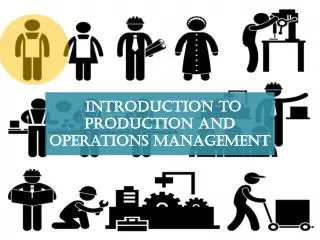
Introduction to Production and Resource Use. Chapter 6. Topics of Discussion. Conditions of perfect competition Classification of productive inputs Important production relationships (Assume one variable input in this chapter) Assessing short run business costs

E N D
Topics of Discussion • Conditions of perfect competition • Classification of productive inputs • Important production relationships (Assume one variable input in this chapter) • Assessing short run business costs • Economics of short run production decisions 2
Conditions for Perfect Competition • Homogeneous products • i.e., Corn grain, mined low-sulfur coal • No barriers to entry or exit • No regulatory barriers • No extremely high fixed costs • Large number of sellers • How large is large? • Perfect information • Information cost is relatively small • No one firm has access to information that others don’t Page 86 3
Classification of Inputs • Economists view the production process as one where a variety of inputs are combined to produce a single or multiple outputs • Cheese plant example • Many inputs: Labor, stainless steel cheese vats, raw milk, energy, starter cultures, cutting and wrapping tables, water, etc. • Multiple outputs: Cheese, dry whey, whey protein concentrates are produced by the plant Pages 86-87 4
Classification of Inputs Land: includes renewable (forests) and non-renewable (minerals) resources Labor: all owner and hired labor services, excluding management Capital: Manufactured goods such as fuel, chemicals, tractors and buildings that may have an extended lifetime Management: Makes production decisions designed to achieve specific economic goals Pages 86-87 5
Classification of Inputs Inputs can also be classified depending on whether amount of input used changes with production level Fixed inputs: The amount of input used does not change with output level Up to a point the size of milking parlor does not change with ↑ milk production/cow or for initial ↑ in herd size Variable Inputs: The amount of input used changes directly with the level of output Usually the amount of labor supplied is a variable input (i.e., car assembly plant that ↑ the speed of assembly line to ↑ production/hour Pages 86-87 6
Production Function “given the level of” Output = f(labor|capital, land, and management) Start with one variable input Assume remaining inputs fixed at current levels • f(•) is general functional notation • Could be any functional form Page 88 7
Production Function • We can graph the relationship between output and amount of labor used • Known as the Total Physical Product (TPP) curve • Purely a physical relationship, no economics involved • X lbs of fertilizer/acre generates a yield of Y Page 89 8
Total Physical Product (TPP) Curve Maximum Output Decreasing output Data from previous table Variable input Page 89 9
Other Physical Relationships • The following derivations of the TPP curve play an important role in decision-making • Marginal Physical Product (MPP) = • Average Physical Product (APP)= Page 90 10
Production Function MPP = Change in output as you change input use ↑MPP ↓MPP Page 89 11
Total Physical Product (TPP) Curve Data from previous table 4.8 • MPP = 1.8/4.0 = .45 • Output ↑ from 3.0 to 4.8 units = 1.8 • Labor ↑ from 16 to 20 units = 4.0 Output 3 Input Page 89 12
Law of DiminishingMarginal Returns • Pertains to what happens to the MPP with increased use of a single variable input • If there are other inputs their level of use is not changed • Diminishing Marginal Returns • The MPP↑ with initial use of a variable input • At some point, MPP reaches a maximum with greater input use • Eventually MPP↓ as input use continues to ↑ Page 93 13
Plotting the MPP Curve Change from A to B on the production function → a MPP of 0.33 Change in output associated with a change in inputs Data from previous table Page 91 15
Plotting the MPP Curve Q of Output MPP = Slope of the line tangent at a point (A) on the TPP curve = ∆Q*/∆I* A ∆Q* Q of Input 0 ∆I* Page 91 16
Plotting the MPP Curve Q of Output At A, MPP = ∆Q/∆I = 0/∆I* = 0 A TPP is at a maximum when MPP = 0 Q of Input 0 ∆I* Page 91 17
Production Function Average Physical Product (APP) = Amount of output ÷ amount of inputs used = Output/unit of input used Page 89 18
Total Physical Product (TPP) Curve Data from previous table Output APP = .31 (= 8÷26) with labor use = 26 Input Page 89 19
Plotting the APP Curve Output divided by labor use at B (3 ÷ 16) =0.19 APP = output level divided by level of input use Data from previous table Page 91 20
Plotting the APP Curve Q of Output B APP = Q*/I* = Slope of the line from the origin to the point on the TPP curve At I**, APP is at a maximum, as line OB is just tangent to the TPP curve A Q* 0 Q of Input I* I** Page 91 21
Relationship Between APP and MPP Q of Output APP is at a maximum at input level where APP = MPP MPP APP* APP Q of Input 0 I* Page 91 22
Definition of the Three Stages of Production Stage I: MPP > APP APP is ↑ APP is increasing in Stage I Page 91 23
Definition of the Three Stages of Production Stage II: MPP < APP MPP > 0 Page 91 24
Definition of the Three Stages of Production Stage III: MPP < 0 Page 91 25
The Three Stages of Production Q of Output MPP APP Stage III Q of Input 0 Stage II Stage I • Stage II starts at input use where APP is at a maximum (pt A) • Stage II ends at input where MPP = 0 (or TPP is at a maximum) Page 91 26
The Three Stages of Production Why are using the amount of input in Stage Iand Stage III of production irrational from the producer’s perspective? Q of Output MPP APP Stage III Q of Input 0 Stage II Stage I Page 91 27
The Three Stages of Production Q of Output Can increase output by using less inputs: →More output and less cost MPP APP Stage III Q of Input 0 Stage II Stage I Average productivity is increasing as more inputs are being used so why stop if the average return is greater than cost? Page 91 28
The Three Stages of Production Q of Output MPP APP Stage III Q of Input 0 Stage II Stage I The producer’s economic question: What level of input amount contained in Stage II should the I use to maximize profits? Page 91 29
Economic Dimension • To answer the above question • We need to account for the price of the product being produced • We also need to account for the cost of the inputs used to produce the above product 30
Key Cost Relationships • The following cost concepts play key roles in determining where in Stage II a producer will want to produce • Total Variable Cost (TVC) = the total value of costs that change with the level of output (e.g. energy costs, labor costs, material costs, etc.) • Total Fixed Cost (TFC) = total value of costs that do not changed with the level of output (e.g. property taxes) • Total Costs (TC) = the sum of total variable and fixed costs • TC = TVC + TFC Page 94-96 31
Key Cost Relationships • The following cost concepts play key roles in determining where in Stage II a producer will want to produce • Marginal Cost (MC) = total cost of production ÷ output produced as output level changes = variable cost of production ÷ output produced given that total fixed costs by definition do not change with output = ∆TC/∆Q = ∆TVC/∆Q • Average Variable Cost (AVC) = total variable cost of production ÷ total amount of output produced = TVC/Q Page 94-96 32
Key Cost Relationships • The following cost concepts play key roles in determining where in Stage II a producer will want to produce • Average Fixed Cost (AFC) = total fixed cost of production ÷ total amount of output produced = TFC/Q • Average Total Cost (ATC) = total cost of production ÷ total amount of output produced = TC/Q = AVC + ATC Page 94-96 33
From TPP curve on page 113 Page 94 34
Fixed costs are $100 no matter the level of production Page 94 35
Total fixed costs (Col. 2) ÷ by total output (Col. 1) Page 94 36
Costs that vary with level of production Page 94 37
Total variable cost (Col. 4) ÷ by total output (Col. 1) 38 Page 94
Total Fixed Cost (Col. 2) + Total Variable Cost (Col.4) Page 94 39
Change in Total Cost (Col. 4 or 6) associated with a change in output (Col. 1) 40 Page 94
[Total Cost (Col. 6) ÷ by Total Output (Col. (1)] or [Avg. Variable Cost + Avg. Fixed Cost] Page 94 41
Let’s Graph the Above Cost Items Contained in the Previous Table 42
Table 6.3 Cost Relationships • MC = min(ATC) and min(AVC) • Vertical distance between ATC and AVC = AFC Cost ($) AFC Input Use Page 95 43
Key Revenue Concepts • The following revenue concepts play key roles in determining where in Stage II a producer will want to produce • Total Revenue (TR) =Multiplication of total amount of output produced by the sale price ($) • Average Revenue (AR) = Total revenue ÷ total amount of output produced ($/unit of output) = TR/Q • Marginal Revenue (MR) = ∆ total revenue ÷ ∆ total amount of output produced = ∆TR÷ ∆Q • How much revenue is generated by one additional unit of output? • Under perfect competition, it is the per unit price 44
Now let’s assume this firm can sell its product for $45/unit 45
Key Revenue Concepts • Remember we are assuming perfect competition • The firm takes price as given • Price (Col. 2) = MR (Col. 7) • What is the AR value? Page 98 46
Profit Maximization • With perfect competition, where would the firm maximize profit in the above example? 47 Page 98
Profit maximizing Output where MR=MC P=MR=AR $45 11.2 Page 99 49
Profit Maximization • The previous graph indicated that • Profit is maximized at 11.2 units of output • MR ($45) equals MC ($45) at 11.2 units of output • Profit maximizing output occurs between points G and H • At 11.2 units of output profit would be $190.40. Let’s do the math…. 50