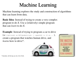
Machine Learning
Machine Learning. Learning from Observations. What is Learning?. Herbert Simon: “Learning is any process by which a system improves performance from experience.”

Machine Learning
E N D
Presentation Transcript
Machine Learning Learning from Observations
What is Learning? Herbert Simon: “Learning is any process by which a system improves performance from experience.” “A computer program is said to learn from experience E with respect to some class of tasks T and performance measure P, if its performance at tasks in T, as measured by P, improves with experience E.” – Tom Mitchell 2
Learning • Learning is essential for unknown environments, • i.e., when designer lacks omniscience • Learning is useful as a system construction method, • i.e., expose the agent to reality rather than trying to write it down • Learning modifies the agent's decision mechanisms to improve performance
Machine Learning • Machine learning: how to acquire a model on the basis of data / experience • Learning parameters (e.g. probabilities) • Learning structure (e.g. BN graphs) • Learning hidden concepts (e.g. clustering)
Machine Learning Areas • Supervised Learning: Data and corresponding labels are given • Unsupervised Learning: Only data is given, no labels provided • Semi-supervised Learning: Some (if not all) labels are present • Reinforcement Learning: An agent interacting with the world makes observations, takes actions, and is rewarded or punished; it should learn to choose actions in such a way as to obtain a lot of reward
Supervised Learning : Important Concepts • Data: labeled instances <xi, y>, e.g. emails marked spam/not spam • Training Set • Held-out Set • Test Set • Features: attribute-value pairs which characterize each x • Experimentation cycle • Learn parameters (e.g. model probabilities) on training set • (Tune hyper-parameters on held-out set) • Compute accuracy of test set • Very important: never “peek” at the test set! • Evaluation • Accuracy: fraction of instances predicted correctly • Overfitting and generalization • Want a classifier which does well on test data • Overfitting: fitting the training data very closely, but not generalizing well
Example: Spam Filter Slide from Mackassy
Example: Digit Recognition Slide from Mackassy
Classification Examples • In classification, we predict labels y (classes) for inputs x • Examples: • OCR (input: images, classes: characters) • Medical diagnosis (input: symptoms, classes: diseases) • Automatic essay grader (input: document, classes: grades) • Fraud detection (input: account activity, classes: fraud / no fraud) • Customer service email routing • Recommended articles in a newspaper, recommended books • DNA and protein sequence identification • Categorization and identification of astronomical images • Financial investments • … many more
Inductive learning • Simplest form: learn a function from examples • f is the target function • An example is a pair (x, f(x)) • Pure induction task: • Given a collection of examples of f, return a function h that approximates f. • find a hypothesis h, such that h ≈ f, given a trainingset of examples • (This is a highly simplified model of real learning: • Ignores prior knowledge • Assumes examples are given)
Inductive learning method • Construct/adjust h to agree with f on training set • (h is consistent if it agrees with f on all examples) • E.g., curve fitting:
Inductive learning method • Construct/adjust h to agree with f on training set • (h is consistent if it agrees with f on all examples) • E.g., curve fitting:
Inductive learning method • Construct/adjust h to agree with f on training set • (h is consistent if it agrees with f on all examples) • E.g., curve fitting:
Inductive learning method • Construct/adjust h to agree with f on training set • (h is consistent if it agrees with f on all examples) • E.g., curve fitting:
Inductive learning method • Construct/adjust h to agree with f on training set • (h is consistent if it agrees with f on all examples) • E.g., curve fitting:
Inductive learning method • Construct/adjust h to agree with f on training set • (h is consistent if it agrees with f on all examples) • E.g., curve fitting: • Ockham’s razor: prefer the simplest hypothesis consistent with data
Generalization Hypotheses must generalize to correctly classify instances not in the training data. Simply memorizing training examples is a consistent hypothesis that does not generalize. Occam’s razor: Finding a simple hypothesis helps ensure generalization. 17
Supervised Learning • Learning a discrete function: Classification • Boolean classification: • Each example is classified as true(positive) or false(negative). • Learning a continuous function: Regression
Classification—A Two-Step Process Model construction: describing a set of predetermined classes Each tuple/sample is assumed to belong to a predefined class, as determined by the class label The set of tuples used for model construction is training set The model is represented as classification rules, decision trees, or mathematical formulae Model usage: for classifying future or unknown objects Estimate accuracy of the model The known label of test sample is compared with the classified result from the model Test set is independent of training set, otherwise over-fitting will occur If the accuracy is acceptable, use the model to classify data tuples whose class labels are not known Data Mining: Concepts and Techniques 20
Issues: Data Preparation Data cleaning Preprocess data in order to reduce noise and handle missing values Relevance analysis (feature selection) Remove the irrelevant or redundant attributes Data transformation Generalize data to (higher concepts, discretization) Normalize attribute values Data Mining: Concepts and Techniques
Classification Techniques • Decision Tree based Methods • Rule-based Methods • Naïve Bayes and Bayesian Belief Networks • Neural Networks • Support Vector Machines • and more...
Learning decision trees Example Problem: decide whether to wait for a table at a restaurant, based on the following attributes: • Alternate: is there an alternative restaurant nearby? • Bar: is there a comfortable bar area to wait in? • Fri/Sat: is today Friday or Saturday? • Hungry: are we hungry? • Patrons: number of people in the restaurant (None, Some, Full) • Price: price range ($, $$, $$$) • Raining: is it raining outside? • Reservation: have we made a reservation? • Type: kind of restaurant (French, Italian, Thai, Burger) • WaitEstimate: estimated waiting time (0-10, 10-30, 30-60, >60)
Feature(Attribute)-based representations • Examples described by feature(attribute) values • (Boolean, discrete, continuous) • E.g., situations where I will/won't wait for a table: • Classification of examples is positive (T) or negative (F)
Decision trees • One possible representation for hypotheses • E.g., here is the “true” tree for deciding whether to wait:
Expressiveness • Decision trees can express any function of the input attributes. • E.g., for Boolean functions, truth table row → path to leaf: • Trivially, there is a consistent decision tree for any training set with one path to leaf for each example (unless f nondeterministic in x) but it probably won't generalize to new examples • Prefer to find more compact decision trees
Decision tree learning • Aim: find a small tree consistent with the training examples • Idea: (recursively) choose "most significant" attribute as root of (sub)tree
Decision Tree Construction Algorithm • Principle • Basic algorithm (adopted by ID3, C4.5 and CART): a greedy algorithm • Tree is constructed in a top-down recursive divide-and-conquer manner • Iterations • At start, all the training tuples are at the root • Tuples are partitioned recursively based on selected attributes • Test attributes are selected on the basis of a heuristic or statistical measure (e.g, information gain) • Stopping conditions • All samples for a given node belong to the same class • There are no remaining attributes for further partitioning – majority voting is employed for classifying the leaf • There are no samples left
Decision Tree Induction: Training Dataset This follows an example of Quinlan’s ID3 (Playing Tennis) September 9, 2014 Data Mining: Concepts and Techniques 30
Tree Induction • Greedy strategy. • Split the records based on an attribute test that optimizes certain criterion. • Issues • Determine how to split the records • How to specify the attribute test condition? • How to determine the best split? • Determine when to stop splitting
Choosing an attribute • Idea: a good attribute splits the examples into subsets that are (ideally) "all positive" or "all negative" • Patrons? is a better choice
How to determine the Best Split • Greedy approach: • Nodes with homogeneous class distribution are preferred • Need a measure of node impurity: Non-homogeneous, High degree of impurity Homogeneous, Low degree of impurity
Measures of Node Impurity • Information Gain • Gini Index • Misclassification error Choose attributes to split to achieve minimum impurity
Attribute Selection Measure: Information Gain (ID3/C4.5) • Select the attribute with the highest information gain • Let pi be the probability that an arbitrary tuple in D belongs to class Ci, estimated by |Ci, D|/|D| • Expected information (entropy) needed to classify a tuple in D: • Information needed (after using A to split D into v partitions) to classify D: • Information gained by branching on attribute A September 9, 2014 Data Mining: Concepts and Techniques 42
Information gain For the training set, p = n = 6, I(6/12, 6/12) = 1 bit Consider the attributes Patrons and Type (and others too): Patrons has the highest IG of all attributes and so is chosen by the DTL algorithm as the root
Example contd. • Decision tree learned from the 12 examples: • Substantially simpler than “true” tree---a more complex hypothesis isn’t justified by small amount of data
Measure of Impurity: GINI (CART, IBM IntelligentMiner) • Gini Index for a given node t : (NOTE: p( j | t) is the relative frequency of class j at node t). • Maximum (1 - 1/nc) when records are equally distributed among all classes, implying least interesting information • Minimum (0.0) when all records belong to one class, implying most interesting information
Splitting Based on GINI • Used in CART, SLIQ, SPRINT. • When a node p is split into k partitions (children), the quality of split is computed as, where, ni = number of records at child i, n = number of records at node p.
Comparison of Attribute Selection Methods The three measures return good results but Information gain: biased towards multivalued attributes Gain ratio: tends to prefer unbalanced splits in which one partition is much smaller than the others Gini index: biased to multivalued attributes has difficulty when # of classes is large tends to favor tests that result in equal-sized partitions and purity in both partitions September 9, 2014 Data Mining: Concepts and Techniques 47
Example Algorithm: C4.5 • Simple depth-first construction. • Uses Information Gain • Sorts Continuous Attributes at each node. • Needs entire data to fit in memory. • Unsuitable for Large Datasets. • You can download the software from Internet
Decision Tree Based Classification • Advantages: • Easy to construct/implement • Extremely fast at classifying unknown records • Models are easy to interpretfor small-sized trees • Accuracy is comparable to other classification techniques for many simple data sets • Tree models make no assumptions about the distribution of the underlying data : nonparametric • Have a built-in feature selection method that makes them immune to the presence of useless variables
Decision Tree Based Classification • Disadvantages • Computationally expensive to train • Some decision trees can be overly complex that do not generalise the data well. • Less expressivity: There may be concepts that are hard to learn with limited decision trees