Download
1 / 22
220 likes | 326 Vues
SOFIE Signal Gain Analysis Mark Hervig GATS. SOFIE Analog Signal Path. Weak Channel Balance Attenuator attenuation = BA w. A/D 14 bits -3V to 3V -2 13 to 2 13 counts 1 count = 366 V. V in,w. Differential Amp gain = G V. Strong Channel Balance Attenuator attenuation = BA s. V in,s.

E N D
SOFIE Analog Signal Path Weak Channel Balance Attenuator attenuation = BAw A/D 14 bits -3V to 3V -213 to 213 counts 1 count = 366 V Vin,w Differential Amp gain = GV Strong Channel Balance Attenuator attenuation = BAs Vin,s • Vin is the signal into the balance attenuator, after synchronous rectification: • Vin = VA/Dmax * margin • set margin to 1.2, so Vin = 3V * 1.2 = 3.6V • we’ll get Vw and Vs below 3V using the BA’s • for example to get Vexo = 2.95V requires BA = 0.82 • The difference signal: • V = (Vin,w * BAw – Vin,s* BAs) * GV
Balance attenuator setting vs. V balance voltages • Difference signal balance voltage, Vbal: • Vbal = (Vin,w * BAw – Vin,s* BAs) * GV • Solve for BAw We can balance at various voltages to increase dynamic range in V Little impact on Vw These curves apply to all channels
V precision vs. V gain and balance attenuator settings count precision, CPV = (214 BAsGV)-1 These curves apply to all channels
V precision vs. balance attenuator setting Count precision, CPV = (214 BA)-1 Lowering BA reduces precision These curves apply to all channels
Recommended V Gain Settings Assumes 14 bit A/D, -3 to 3V. V balance voltage was –2.5V for all channels. Upper altitude is where the 1st 10 count change occurs. Lower altitude is where V reaches 0.8214 counts. Note that the CBE 1-count precisions are not CBE system noise. Required V precisions are taken as the strong band requirements. Signals were based on atmospheric transmissions calculated using a climatology for summer at 60°N. The analyses that lead to the above results are shown on the following pages.
(Chad) SOFIE Radiometric Measurement End-to-End Required SNRs
SOFIE PC Radiometric Electronics Overview • Carrier Frequency = 1kHz, Modulation = 2 Hz, Effective Sync Rect Q = 500 • Nominal Equal System-wide Phasing: Butterworth and Bessel Filters
1) O3 channel profiles Balance V at –2.5V BAs = 0.819 BAw = 0.613 GV = 3.3 V saturates at 60 km, or 0.8*214 counts
1) O3 Channel useful altitude Useful altitude of V signals is determined by the V gain and balance attenuator settings. Baseline altitude range will be determined by GV Adjusting the BA settings changes the altitude range very little in this case
2) SW particle channel profiles Balance V at –2.5V BAs = 0.819 BAw = 0.814 GV = 300 V useable through typical PMC
3) H2O channel profiles Balance V at –2.5V BAs = 0.819 BAw = 0.812 GV = 96 V saturates at 50 km, or 0.8*214 counts
3) H2O Channel useful altitude Useful altitude of V signals is determined by the V gain and balance attenuator settings. Baseline altitude range will be determined by GV We can adjust the BA settings to change our altitude range
3) H2O channel useful altitude The V gain to saturate at 50 km altitude changes with V balance voltage Decreasing the V balance voltage increases the dynamic range With increased dynamic range, we can tolerate an increase in the V gain The figure shows the V gain that saturates V at 50 km vs. Vbal Decreasing Vbal allows us to get more precision and dynamic range
4) 2.8 m CO2 channel useful altitude Useful altitude of V signals is determined by the V gain and balance attenuator settings. Baseline altitude range will be determined by GV Adjusting the BA settings changes the altitude range
5) IR particle channel profiles Balance V at –2.5V BAs = 0.819 BAw = 0.814 GV = 120 V useable through typical PMC
6) CH4 channel profiles Balance V at –2.5V BAs = 0.819 BAw = 0.816 GV = 202 V saturates at 40 km, or 0.8*214 counts
6) CH4 Channel useful altitude Useful altitude of V signals is determined by the V gain and balance attenuator settings. Baseline altitude range will be determined by GV Adjusting the BA settings changes the altitude range
7) 4.3 m CO2 channel useful altitude Useful altitude of V signals is determined by the V gain and balance attenuator settings. Baseline altitude range will be determined by GV Adjusting the BA settings changes the altitude range
8) NO channel profiles Balance V at –2.5V BAs = 0.819 BAw = 0.817 GV = 300 V never saturates, but the signal is dominated by atmospheric interference below 80 km.