Frequent Pattern Analysis in Data Mining
880 likes | 996 Vues
Explore the concept of frequent patterns, itemsets, and association rules in data mining for uncovering regularities and insights in various data sets. Discover applications and methods like Apriori algorithm for efficient pattern mining.

Frequent Pattern Analysis in Data Mining
E N D
Presentation Transcript
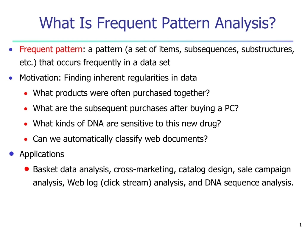
What Is Frequent Pattern Analysis? • Frequent pattern: a pattern (a set of items, subsequences, substructures, etc.) that occurs frequently in a data set • Motivation: Finding inherent regularities in data • What products were often purchased together? • What are the subsequent purchases after buying a PC? • What kinds of DNA are sensitive to this new drug? • Can we automatically classify web documents? • Applications • Basket data analysis, cross-marketing, catalog design, sale campaign analysis, Web log (click stream) analysis, and DNA sequence analysis.
Frequent item sets • Set of items – itemset • Itemset with ‘k’ items is called ‘k-itemset’ • Occurrence of itemset – number of transactions that contain the itemset (frequency) • If the support of an itemset satisfies a minimum support threshold then it is called as frequent itemset Confidence(A=>B) = P(B|A) = support(AUB)/Support A
Customer buys both Customer buys diaper Customer buys beer Basic Concepts: Frequent Patterns and Association Rules • Itemset X = {x1, …, xk} • Find all the rules X Ywith minimum support and confidence • support, s, probability that a transaction contains X Y • confidence, c,conditional probability that a transaction having X also contains Y • Let supmin = 50%, confmin = 50% • Freq. Pat.: {A:3, B:3, D:4, E:3, AD:3} • Association rules: • A D (60%, 100%) • D A (60%, 75%)
Two – step process of association mining • Find all frequent itemsets: more than min-support • Generate strong association rules from the frequent itemsets: rules that support minimum support and minimum confidence Data Mining: Concepts and Techniques
Closed Patterns and Max-Patterns • A long pattern contains a combinatorial number of sub-patterns, e.g., {a1, …, a100} contains (1001) + (1002) + … + (110000) = 2100 – 1 = 1.27*1030 sub-patterns! • Solution: Mine closed patterns and max-patterns instead • An itemset Xis closed if X is frequent and there exists no super-pattern Y כ X, with the same support as X • An itemset X is a max-pattern if X is frequent and there exists no frequent super-pattern Y כ X • Closed pattern is a lossless compression of freq. patterns • Reducing the # of patterns and rules
Scalable Methods for Mining Frequent Patterns • The downward closure property of frequent patterns • Any subset of a frequent itemset must be frequent • If {beer, diaper, nuts} is frequent, so is {beer, diaper} • i.e., every transaction having {beer, diaper, nuts} also contains {beer, diaper} • Scalable mining methods: Three major approaches • Apriori (Agrawal & Srikant@VLDB’94) • Freq. pattern growth (FPgrowth—Han, Pei & Yin @SIGMOD’00) • Vertical data format approach (Charm—Zaki & Hsiao @SDM’02)
Frequent pattern mining • Frequent pattern mining can be classified in various ways • Based on the completeness of pattern to be mined • Based on the levels of abstraction • Based on the number of data dimension • Based on the types of values • Based on the kinds of rules to be mining • Based on the kinds of patterns to be mined
Apriori: A Candidate Generation-and-Test Approach • Apriori pruning principle: If there is any itemset which is infrequent, its superset should not be generated/tested! (Agrawal & Srikant @VLDB’94, Mannila, et al. @ KDD’ 94) • Method: • Initially, scan DB once to get frequent 1-itemset • Generate length (k+1) candidate itemsets from length k frequent itemsets • Test the candidates against DB • Terminate when no frequent or candidate set can be generated
The Apriori Algorithm—An Example Supmin = 2 Database TDB L1 C1 1st scan C2 C2 L2 2nd scan L3 C3 3rd scan Data Mining: Concepts and Techniques
The Apriori Algorithm • Pseudo-code: Ck: Candidate itemset of size k Lk : frequent itemset of size k L1 = {frequent items}; for(k = 1; Lk !=; k++) do begin Ck+1 = candidates generated from Lk; for each transaction t in database do increment the count of all candidates in Ck+1 that are contained in t Lk+1 = candidates in Ck+1 with min_support end returnkLk; Data Mining: Concepts and Techniques
Important Details of Apriori • How to generate candidates? • Step 1: self-joining Lk • Step 2: pruning • How to count supports of candidates? • Example of Candidate-generation • L3={abc, abd, acd, ace, bcd} • Self-joining: L3*L3 • abcd from abc and abd • acde from acd and ace • Pruning: • acde is removed because ade is not in L3 • C4={abcd} Data Mining: Concepts and Techniques
How to Count Supports of Candidates? • Why counting supports of candidates a problem? • The total number of candidates can be very huge • One transaction may contain many candidates • Method: • Candidate itemsets are stored in a hash-tree • Leaf node of hash-tree contains a list of itemsets and counts • Interior node contains a hash table • Subset function: finds all the candidates contained in a transaction Data Mining: Concepts and Techniques
Generating Association Rules from Frequent Itemsets • Strong association rules satisfy both minimum support and minimum confidence • For each frequent itemsetl, generate all nonempty sunsets of l. • For every nonempty subset s of l, output the rule “s=>(l-s)” if support_count(l)/support_count(s)>=min_conf where min_conf is the minimum confidence threshold Data Mining: Concepts and Techniques
Generating Association rules • Considering the frequent itemset l={I1,I2,I5} and minimum confidence is 70% find the strong association rules
Improving the efficiency of apriori • Hash-based technique: While generating the candidate 1- itemsets , we can generate all of the 2-itemsets for each transaction, hash them into different buckets of a hash table structure and increase the corresponding bucket counts • Transaction Reduction: if transaction does not contain frequent k-itemsets cannot contain any (k+1) itemsets
Improving the efficiency of Apriori • Partitioning: • Requires two database scans • Consists of two phases • Phase I: divides the transactions into n nonoverlapping partitions (min sup=min_sup* # transactions). Local frequent itemsets are found • Any itemset frequent in D should be frequent in atleast one partition • Phase II: scan D to determine the actual support of each candidate to access the global frequent itemsets.
Improving the efficiency of Apriori • Sampling: • Pick a random sample S of D, search for frequent itemsets in S • To lessen the possibility of missing some global frequent itemsets lower the minimum support • Rest of database is then checked to find the actual frequencies of each itemset. • If the min support of the sample contains all the frequent itemsets in D then only one scan of D is required
Dynamic itemset counting • In this technique candidate itemsets is added at different points during a scan • Dbase is partitioned into blocks marked by start points • New candidate itemsets can be added at any start point • Algo requires fewer database scans than apriori Data Mining: Concepts and Techniques
Challenges of Frequent Pattern Mining • Challenges • Multiple scans of transaction database • Huge number of candidates • Tedious workload of support counting for candidates • Improving Apriori: general ideas • Reduce passes of transaction database scans • Shrink number of candidates • Facilitate support counting of candidates Data Mining: Concepts and Techniques
Partition: Scan Database Only Twice • Any itemset that is potentially frequent in DB must be frequent in at least one of the partitions of DB • Scan 1: partition database and find local frequent patterns • Scan 2: consolidate global frequent patterns • A. Savasere, E. Omiecinski, and S. Navathe. An efficient algorithm for mining association in large databases. In VLDB’95 Data Mining: Concepts and Techniques
DHP: Reduce the Number of Candidates • A k-itemset whose corresponding hashing bucket count is below the threshold cannot be frequent • Candidates: a, b, c, d, e • Hash entries: {ab, ad, ae} {bd, be, de} … • Frequent 1-itemset: a, b, d, e • ab is not a candidate 2-itemset if the sum of count of {ab, ad, ae} is below support threshold • J. Park, M. Chen, and P. Yu. An effective hash-based algorithm for mining association rules. In SIGMOD’95 Data Mining: Concepts and Techniques
Sampling for Frequent Patterns • Select a sample of original database, mine frequent patterns within sample using Apriori • Scan database once to verify frequent itemsets found in sample, only bordersof closure of frequent patterns are checked • Example: check abcd instead of ab, ac, …, etc. • Scan database again to find missed frequent patterns • H. Toivonen. Sampling large databases for association rules. In VLDB’96 Data Mining: Concepts and Techniques
Once both A and D are determined frequent, the counting of AD begins Once all length-2 subsets of BCD are determined frequent, the counting of BCD begins DIC: Reduce Number of Scans ABCD ABC ABD ACD BCD AB AC BC AD BD CD Transactions 1-itemsets B C D A 2-itemsets Apriori … {} Itemset lattice 1-itemsets S. Brin R. Motwani, J. Ullman, and S. Tsur. Dynamic itemset counting and implication rules for market basket data. In SIGMOD’97 2-items DIC 3-items Data Mining: Concepts and Techniques
Bottleneck of Frequent-pattern Mining • Multiple database scans are costly • Mining long patterns needs many passes of scanning and generates lots of candidates • To find frequent itemset i1i2…i100 • # of scans: 100 • # of Candidates: (1001) + (1002) + … + (110000) = 2100-1 = 1.27*1030 ! • Bottleneck: candidate-generation-and-test • Can we avoid candidate generation? Data Mining: Concepts and Techniques
Mining Frequent Patterns WithoutCandidate Generation • Grow long patterns from short ones using local frequent items • “abc” is a frequent pattern • Get all transactions having “abc”: DB|abc • “d” is a local frequent item in DB|abc abcd is a frequent pattern Data Mining: Concepts and Techniques
{} Header Table Item frequency head f 4 c 4 a 3 b 3 m 3 p 3 f:4 c:1 c:3 b:1 b:1 a:3 p:1 m:2 b:1 p:2 m:1 Construct FP-tree from a Transaction Database TID Items bought (ordered) frequent items 100 {f, a, c, d, g, i, m, p}{f, c, a, m, p} 200 {a, b, c, f, l, m, o}{f, c, a, b, m} 300 {b, f, h, j, o, w}{f, b} 400 {b, c, k, s, p}{c, b, p} 500{a, f, c, e, l, p, m, n}{f, c, a, m, p} min_support = 3 • Scan DB once, find frequent 1-itemset (single item pattern) • Sort frequent items in frequency descending order, f-list • Scan DB again, construct FP-tree F-list=f-c-a-b-m-p Data Mining: Concepts and Techniques
Benefits of the FP-tree Structure • Completeness • Preserve complete information for frequent pattern mining • Never break a long pattern of any transaction • Compactness • Reduce irrelevant info—infrequent items are gone • Items in frequency descending order: the more frequently occurring, the more likely to be shared • Never be larger than the original database (not count node-links and the count field) • For Connect-4 DB, compression ratio could be over 100 Data Mining: Concepts and Techniques
Partition Patterns and Databases • Frequent patterns can be partitioned into subsets according to f-list • F-list=f-c-a-b-m-p • Patterns containing p • Patterns having m but no p • … • Patterns having c but no a nor b, m, p • Pattern f • Completeness and non-redundency Data Mining: Concepts and Techniques
{} Header Table Item frequency head f 4 c 4 a 3 b 3 m 3 p 3 f:4 c:1 c:3 b:1 b:1 a:3 p:1 m:2 b:1 p:2 m:1 Find Patterns Having P From P-conditional Database • Starting at the frequent item header table in the FP-tree • Traverse the FP-tree by following the link of each frequent item p • Accumulate all of transformed prefix paths of item p to form p’s conditional pattern base Conditional pattern bases item cond. pattern base c f:3 a fc:3 b fca:1, f:1, c:1 m fca:2, fcab:1 p fcam:2, cb:1 Data Mining: Concepts and Techniques
{} f:3 c:3 a:3 m-conditional FP-tree From Conditional Pattern-bases to Conditional FP-trees • For each pattern-base • Accumulate the count for each item in the base • Construct the FP-tree for the frequent items of the pattern base • m-conditional pattern base: • fca:2, fcab:1 {} Header Table Item frequency head f 4 c 4 a 3 b 3 m 3 p 3 All frequent patterns relate to m m, fm, cm, am, fcm, fam, cam, fcam f:4 c:1 c:3 b:1 b:1 a:3 p:1 m:2 b:1 p:2 m:1 Data Mining: Concepts and Techniques
{} f:3 c:3 am-conditional FP-tree {} f:3 c:3 a:3 m-conditional FP-tree Recursion: Mining Each Conditional FP-tree Cond. pattern base of “am”: (fc:3) {} Cond. pattern base of “cm”: (f:3) f:3 cm-conditional FP-tree {} Cond. pattern base of “cam”: (f:3) f:3 cam-conditional FP-tree Data Mining: Concepts and Techniques
a1:n1 a1:n1 {} {} a2:n2 a2:n2 a3:n3 a3:n3 r1 C1:k1 C1:k1 r1 = b1:m1 b1:m1 C2:k2 C2:k2 C3:k3 C3:k3 A Special Case: Single Prefix Path in FP-tree • Suppose a (conditional) FP-tree T has a shared single prefix-path P • Mining can be decomposed into two parts • Reduction of the single prefix path into one node • Concatenation of the mining results of the two parts + Data Mining: Concepts and Techniques
Mining Frequent Patterns With FP-trees • Idea: Frequent pattern growth • Recursively grow frequent patterns by pattern and database partition • Method • For each frequent item, construct its conditional pattern-base, and then its conditional FP-tree • Repeat the process on each newly created conditional FP-tree • Until the resulting FP-tree is empty, or it contains only one path—single path will generate all the combinations of its sub-paths, each of which is a frequent pattern Data Mining: Concepts and Techniques
Scaling FP-growth by DB Projection • FP-tree cannot fit in memory?—DB projection • First partition a database into a set of projected DBs • Then construct and mine FP-tree for each projected DB • Parallel projection vs. Partition projection techniques • Parallel projection is space costly Data Mining: Concepts and Techniques
Tran. DB fcamp fcabm fb cbp fcamp p-proj DB fcam cb fcam m-proj DB fcab fca fca b-proj DB f cb … a-proj DB fc … c-proj DB f … f-proj DB … am-proj DB fc fc fc cm-proj DB f f f … Partition-based Projection • Parallel projection needs a lot of disk space • Partition projection saves it Data Mining: Concepts and Techniques
FP-Growth vs. Apriori: Scalability With the Support Threshold Data set T25I20D10K Data Mining: Concepts and Techniques
FP-Growth vs. Tree-Projection: Scalability with the Support Threshold Data set T25I20D100K Data Mining: Concepts and Techniques
Why Is FP-Growth the Winner? • Divide-and-conquer: • decompose both the mining task and DB according to the frequent patterns obtained so far • leads to focused search of smaller databases • Other factors • no candidate generation, no candidate test • compressed database: FP-tree structure • no repeated scan of entire database • basic ops—counting local freq items and building sub FP-tree, no pattern search and matching Data Mining: Concepts and Techniques
Implications of the Methodology • Mining closed frequent itemsets and max-patterns • CLOSET (DMKD’00) • Mining sequential patterns • FreeSpan (KDD’00), PrefixSpan (ICDE’01) • Constraint-based mining of frequent patterns • Convertible constraints (KDD’00, ICDE’01) • Computing iceberg data cubes with complex measures • H-tree and H-cubing algorithm (SIGMOD’01) Data Mining: Concepts and Techniques
MaxMiner: Mining Max-patterns • 1st scan: find frequent items • A, B, C, D, E • 2nd scan: find support for • AB, AC, AD, AE, ABCDE • BC, BD, BE, BCDE • CD, CE, CDE, DE, • Since BCDE is a max-pattern, no need to check BCD, BDE, CDE in later scan • R. Bayardo. Efficiently mining long patterns from databases. In SIGMOD’98 Potential max-patterns Data Mining: Concepts and Techniques
Mining Frequent Closed Patterns: CLOSET • Flist: list of all frequent items in support ascending order • Flist: d-a-f-e-c • Divide search space • Patterns having d • Patterns having d but no a, etc. • Find frequent closed pattern recursively • Every transaction having d also has cfa cfad is a frequent closed pattern • J. Pei, J. Han & R. Mao. CLOSET: An Efficient Algorithm for Mining Frequent Closed Itemsets", DMKD'00. Min_sup=2 Data Mining: Concepts and Techniques
CLOSET+: Mining Closed Itemsets by Pattern-Growth • Itemset merging: if Y appears in every occurrence of X, then Y is merged with X • Sub-itemset pruning: if Y כ X, and sup(X) = sup(Y), X and all of X’s descendants in the set enumeration tree can be pruned • Hybrid tree projection • Bottom-up physical tree-projection • Top-down pseudo tree-projection • Item skipping: if a local frequent item has the same support in several header tables at different levels, one can prune it from the header table at higher levels • Efficient subset checking Data Mining: Concepts and Techniques
CHARM: Mining by Exploring Vertical Data Format • Vertical format: t(AB) = {T11, T25, …} • tid-list: list of trans.-ids containing an itemset • Deriving closed patterns based on vertical intersections • t(X) = t(Y): X and Y always happen together • t(X) t(Y): transaction having X always has Y • Using diffset to accelerate mining • Only keep track of differences of tids • t(X) = {T1, T2, T3}, t(XY) = {T1, T3} • Diffset (XY, X) = {T2} • Eclat/MaxEclat (Zaki et al. @KDD’97), VIPER(P. Shenoy et al.@SIGMOD’00), CHARM (Zaki & Hsiao@SDM’02) Data Mining: Concepts and Techniques
Further Improvements of Mining Methods • AFOPT (Liu, et al. @ KDD’03) • A “push-right” method for mining condensed frequent pattern (CFP) tree • Carpenter (Pan, et al. @ KDD’03) • Mine data sets with small rows but numerous columns • Construct a row-enumeration tree for efficient mining Data Mining: Concepts and Techniques
