Discriminative Frequent Pattern Analysis for Effective Classification
This presentation discusses a novel framework for classification utilizing discriminative frequent patterns to improve both scalability and accuracy in large datasets. It addresses the motivation for using frequent patterns, their effectiveness as a substitute for complete pattern sets, and strategies for setting minimum support thresholds. Key definitions such as Fisher Score and Information Gain are detailed, alongside methods for generating and selecting high-quality features. The authors propose an efficient feature selection algorithm and validate the performance through experiments with SVM and C4.5 classifiers.

Discriminative Frequent Pattern Analysis for Effective Classification
E N D
Presentation Transcript
Discriminative Frequent Pattern Analysis for Effective Classification By Hong Cheng, Xifeng Yan, Jiawei Han, Chih-Wei Hsu Presented by Mary Biddle
Patterns ABCD ABCF BCD BCEF Frequency A = 2 B = 4 C = 4 D = 2 E = 1 F = 2 AB = 2 BC = 4 CD = 2 CE = 1 CF = 2 IntroductionPattern Example
Motivation • Why are frequent patterns useful for classification? Why do frequent patterns provide a good substitute for the complete pattern set? • How does frequent pattern-based classification achieve both high scalabilityand accuracy for the classification of large datasets? • What is the strategy for setting the minimum support threshold? • Given a set of frequent patterns, how should we select high quality ones for effective classification?
InformationFisher Score Definition • In statistics and information theory, the Fisher Information is the variance of the score. • The Fisher information is a way of measuring the amount of information that an observable random variable X carries about an unknown parameter θ upon which the likelihood function of θ, L(θ) = f(X, θ), depends. The likelihood function is the joint probability of the data, the Xs, conditional on the value of θ, as a function of θ.
IntroductionInformation Gain Definition • In probability theory and information theory Information Gain is a measure of the difference between two probability distributions: from a “true” probability distribution P to an arbitrary probability distribution Q. • The expected Information Gain is the change in information entropy from a prior state to a state that take some information as given. • Usually an attribute with high information gain should be preferred to other attributes.
ModelCombined Feature Definition • Each (attribute, value) pair is mapped to a distinct item in I = {o1,…,od}. • A combined feature α = {oα1,…,oαk} is a subset of I, where oαi{o1,…,od}, 1 ≤ i ≤ k • oiI is a single feature. • Given a dataset D = {xi}, the set of data that contains α is denoted as Dα = {xi|xiαj = 1, oαj α}.
ModelFrequent Combined Feature Definition • For a dataset D, a combined feature α is frequent if θ = |Dα|/|D| ≥ θ0, whereθ is the relative support of α, and θ0 is the min_sup threshold, 0 ≤ θ0 ≤ 1. • The set of frequent defined features is denoted as F.
ModelInformation Gain • For a patter α represented by a random variable X, the information gain is IG(C|X) = H(C)-H(C|X) • Where H(C) is the entropy • And H(C|X) is the conditional entropy • Given a dataset with a fixed class distribution, H(C) is a constant.
The information gain upper bound IGub is IGub(C|X) = H(C) - Hlb(C|X) Where Hlb is the lower bound ofH(C|X) Model Information Gain Upper Bound
ModelFisher Score • Fisher score is defined as Fr = (∑ci=1 ni(uui-u)2)/ (∑ci=1 niσi2) • where ni is the number of data samples in class i, • uui is the average feature value in class i • σi is the standard deviation of the feature value in class i • u is the average feature value in the whole dataset.
ModelRelevance Measure S • A relevance measure S is a function mapping a pattern αto a real value such that S(α) is the relevance w.r.t. the class label. • Measures like information gain and fisher score can be used as a relevance measure.
ModelRedundancy Measure • A redundancy measure R is a function mapping two patterns αand ß to a real value such that R(α, ß) is the redundancy between them. • R(α, ß) = (P(α, ß) / (P(α) + P(ß) – P(α,ß) ))x min(S(α),S(ß)) P is the predicate function from the Jaccard measure.
Modelinformation gain • The gain of a pattern α given a set of already selected patterns Fs is • g(α)=S(α)-maxR(α, ß) • Where ß Fs
Algorithm framework of frequent pattern-based classification • Feature generation • Feature selection • Model learning
Algorithm1. Feature Generation • Compute information gain (or Fisher score) upper bound as a function of support θ. • Choose an information gain threshold IG0 for feature filtering purposes. • Find θ* = arg maxθ (IGub(θ)≤IG0) • Mine frequent patterns with min_sup = θ*
Algorithm3. Model Learning • Use the resulting features as input to the learning model of your choice. • They experimented with SVM and C4.5
Contributions • Propose a framework of frequent pattern-based classification by analyzing the relationship between pattern frequency and its predictive power. • Frequent pattern-based classification could exploit the state-of-the-art frequent pattern mining algorithms for feature generation with much better scalability. • Suggest a strategy for setting a minimum support. • An effective and efficient feature selection algorithm is proposed to select a set of frequent and discriminative patterns for classification.
Related Work • Associative Classification • The association between frequent patterns and class labels is used for prediction. A classifier is built based on high-confidence, high-support association rules. • Top-K rule mining • A recent work on top-k rule mining discovers top-k covering rule groups for each row of gene expression profiles. Prediction is perfomed based on a classification score which combines the support and confidence measures of the rules. • HARMONY (mines classification rules) • It uses an instance-centric rule-generation approach and assures for each training instance, that one of the highest confidence rules covering the instance is included in the rule set. This is the more efficient and scalable than previous rule-based classifiers. On several datasets the classifier accuracy was significantly higher, i.e. 11.94% on Waveform and 3.4% on Letter Recognition. • All of the following use frequent patterns • String kernels • Word combinations (NLP) • Structural features in graph classification
Differences betweenAssociative ClassificationandDiscriminative Frequent Pattern Analysis Classification • Frequent Patterns are used to represent the data in a different feature space. Associative classification builds a classification using rules only. • In associative classification, the prediction process is to find one or several top ranked rule(s) for prediction. In this process, the prediction is made by the classification model. • The information gain is used to discriminate the patterns being used by using it to determine the min_sup and in the selection of the frequent patterns.
Pros Reduces Time More accurate Cons Space concerns on large datasets because it uses the entire Pattern set, initially. Pros and Cons