Download
1 / 25
250 likes | 273 Vues
Understand generative vs. discriminative classification methods, advantages of discriminative models, linear classifiers, logistic discriminant for multiple classes, and parameter estimation.

E N D
Classification 2: discriminative models Jakob Verbeek January 14, 2011 SVM slides stolen from Svetlana Lazebnik Course website: http://lear.inrialpes.fr/~verbeek/MLCR.10.11.php
Plan for the course • Session 4, December 17 2010 • Jakob Verbeek: The EM algorithm, and Fisher vector image representation • Cordelia Schmid: Bag-of-features models for category-level classification • Student presentation 2: Beyond bags of features: spatial pyramid matching for recognizing natural scene categories, Lazebnik, Schmid and Ponce, CVPR 2006. • Session 5, January 7 2011 • Jakob Verbeek: Classification 1: generative and non-parameteric methods • Student presentation 4: Large-Scale Image Retrieval with Compressed Fisher Vectors, Perronnin, Liu, Sanchez and Poirier, CVPR 2010. • Cordelia Schmid: Category level localization: Sliding window and shape model • Student presentation 5: Object Detection with Discriminatively Trained Part Based Models, Felzenszwalb, Girshick, McAllester and Ramanan, PAMI 2010. • Session 6, January 14 2011 • Jakob Verbeek: Classification 2: discriminative models • Student presentation 6:TagProp: Discriminative metric learning in nearest neighbor models for image auto-annotation, Guillaumin, Mensink, Verbeek and Schmid, ICCV 2009. • Student presentation 7:IM2GPS: estimating geographic information from a single image, Hays and Efros, CVPR 2008.
Example of classification apple pear tomato cow dog horse Given: training images x and their categories y What are the categories of these test images?
Generative vs Discriminative Classification Training data consists of “inputs”, denoted x, and corresponding output “class labels”, denoted as y. Goal is to predict class label y for a given test data x. Generative probabilistic methods Model the density of inputs x from each class p(x|y) Estimate class prior probability p(y) Use Bayes’ rule to infer distribution over class given input Discriminative (probabilistic) methods Directly estimate class probability given input: p(y|x) Some methods do not have probabilistic interpretation, but fit a function f(x), and assign to classes based on sign(f(x))
Choose class of decision functions in feature space. Estimate the function parameters from the training set. Classify a new pattern on the basis of this decision rule. Discriminant function kNN example from last week Needs to store all data Separation using smooth curve Only need to store curve parameters
Linear classifiers Decision function is linear in the features: Classification based on the sign of f(x) Orientation is determined by w (surface normal) Offset from origin is determined by w0 Decision surface is (d-1) dimensional hyper-plane orthogonal to w, given by f(x)=0 w
Linear classifiers Decision function is linear in the features: Classification based on the sign of f(x) Orientation is determined by w (surface normal) Offset from origin is determined by w0 Decision surface is (d-1) dimensional hyper-plane orthogonal to w, given by What happens in 3d with w=(1,0,0) and w0 =-1 ? f(x)=0 w
Dealing with more than two classes First (bad) idea: construction from multiple binary classifiers Learn the 2-class “base” classifiers independently One vs rest classifiers: train 1 vs (2 & 3), and 2 vs (1 & 3), and 3 vs (1 & 2) One vs One classifiers: train 1 vs 2, and 2 vs 3 and 1 vs 3 Not clear what should be done in some regions One vs Rest: Region claimed by several classes One vs One: no agreement
Dealing with more than two classes Alternative: define a separate linear function for each class Assign sample to the class of the function with maximum value Decision regions are convex in this case If two points fall in the region, then also all points on connecting line What shape do the separation surfaces have ?
Logistic discriminant for two classes Map linear score function to class probabilities with sigmoid function The class boundary is obtained for p(y|x)=1/2, thus by setting linear function in exponent to zero f(x)=+5 p(y|x)=1/2 f(x)=-5 w
Multi-class logistic discriminant Map K linear score functions (one for each class) to K class probabilities using the “soft-max” function The class probability estimates are non-negative, and sum to one. Probability for the most likely class increases quickly with the difference in the linear score functions For any given pair of classes we find that they are equally likely on a hyperplane in the feature space
Parameter estimation for logistic discriminant Maximize the (log) likelihood of predicting the correct class label for training data, ie the sum log-likelihood of all training data Derivative of log-likelihood as intuitive interpretation No closed-form solution, use gradient-descent methods Note 1: log-likelihood is concave in parameters, hence no local optima Note 2: w is linear combination of data points Indicator function 1 if yn=c, else 0 Expected number of points from each class should equal the actual number. Expected value of each feature, weighting points by p(y|x), should equal empirical expectation.
Support Vector Machines • Find linear function (hyperplane) to separate positive and negative examples Which hyperplaneis best?
Support vector machines • Find hyperplane that maximizes the margin between the positive and negative examples C. Burges, A Tutorial on Support Vector Machines for Pattern Recognition, Data Mining and Knowledge Discovery, 1998
Support vector machines • Find hyperplane that maximizes the margin between the positive and negative examples For support vectors, Distance between point and hyperplane: Therefore, the margin is 2 / ||w|| Support vectors Margin C. Burges, A Tutorial on Support Vector Machines for Pattern Recognition, Data Mining and Knowledge Discovery, 1998
Finding the maximum margin hyperplane • Maximize margin 2/||w|| • Correctly classify all training data: • Quadratic optimization problem: • Minimize Subject to yi(w·xi+b) ≥ 1 C. Burges, A Tutorial on Support Vector Machines for Pattern Recognition, Data Mining and Knowledge Discovery, 1998
Finding the maximum margin hyperplane • Solution: learnedweight Support vector C. Burges, A Tutorial on Support Vector Machines for Pattern Recognition, Data Mining and Knowledge Discovery, 1998
Finding the maximum margin hyperplane • Solution:b = yi – w·xi for any support vector • Classification function (decision boundary): • Notice that it relies on an inner product between the testpoint xand the support vectors xi • Solving the optimization problem also involvescomputing the inner products xi· xjbetween all pairs oftraining points C. Burges, A Tutorial on Support Vector Machines for Pattern Recognition, Data Mining and Knowledge Discovery, 1998
Summary Linear discriminant analysis Two most widely used linear classifiers in practice: Logistic discriminant (supports more than 2 classes directly) Support vector machines (multi-class extensions recently developed) In both cases the weight vector w is a linear combination of the data points This means that we only need the inner-products between data points to calculate the linear functions The function k that computes the inner products is called a kernel function
x 0 x 0 x2 Nonlinear SVMs • Datasets that are linearly separable work out great: • But what if the dataset is just too hard? • We can map it to a higher-dimensional space: 0 x Slide credit: Andrew Moore
Nonlinear SVMs • General idea: the original input space can always be mapped to some higher-dimensional feature space where the training set is separable: Φ: x→φ(x) Slide credit: Andrew Moore
Nonlinear SVMs • The kernel trick: instead of explicitly computing the lifting transformation φ(x), define a kernel function K such thatK(xi,xj) = φ(xi)· φ(xj) • (to be valid, the kernel function must satisfy Mercer’s condition) • This gives a nonlinear decision boundary in the original feature space: C. Burges, A Tutorial on Support Vector Machines for Pattern Recognition, Data Mining and Knowledge Discovery, 1998
Kernels for bags of features • Histogram intersection kernel: • Generalized Gaussian kernel: • D can be Euclidean distance, χ2distance,Earth Mover’s Distance, etc. J. Zhang, M. Marszalek, S. Lazebnik, and C. Schmid, Local Features and Kernels for Classifcation of Texture and Object Categories: A Comprehensive Study, IJCV 2007
Summary: SVMs for image classification • Pick an image representation (in our case, bag of features) • Pick a kernel function for that representation • Compute the matrix of kernel values between every pair of training examples • Feed the kernel matrix into your favorite SVM solver to obtain support vectors and weights • At test time: compute kernel values for your test example and each support vector, and combine them with the learned weights to get the value of the decision function
SVMs vs Logisitic discriminants • Multi-class SVMs can be obtained in a similar way as for logistic discriminants • Separate linear score function for each class • Kernels can also be used for non-linear logisitic discriminants • Requires storing the support vectors, may cost lots of memory in practice • Computing kernel between new data point and support vectors may be computationally expensive • For Logisitic discriminant to work well in practice with small number of examples, regularizer needs to be added to achieve large margins • Kernel functions can be applied to virtually any linear data processing technique • Principle component analysis, k-means clustering, ….