Cloud Processes in Climate System: Some Research Topics

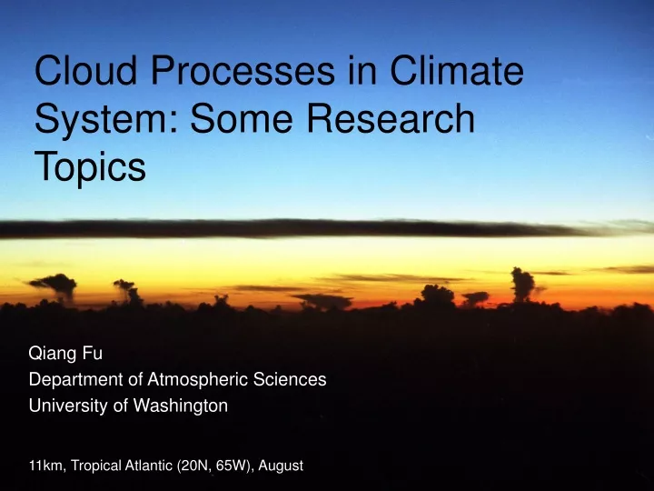
1. Cloud Processes in Climate System: Some Research Topics Qiang Fu Department of Atmospheric Sciences University of Washington 11km, Tropical Atlantic (20N, 65W), August

2. Response of a Climate Model to 2xCO2

3. TOPICS • Testing Mixed-Phase Cloud Water Vapor Parameterizations with SHEBA/FIRE-ACE Observations • Tests and Improvements of GCM Cloud Parameterizations Using the CCCMA SCM with the SHEBA Dataset • Radiative Energy Balance in the Tropical Upper Troposphere

4. GCM Cloud Responses to 2xCO2 Senior et al. (1993)

5. Saturated Water Vapor Pressure Fu and Hollars (2004)

6. Parameterization of Es in Numerical Models: • Saturated water vapor pressure, Es, can be written as • Es = REsl + (1-R)Esi • where Esl and Esi are the saturated vapor pressure • with respect to water and ice, respectively. • R(T) R = [ (T + 23) /23 ]2, –23oC < T < 0oC (ECMWF) • R = (T+20)/20, –20oC < T < 0oC (Fowler et al. 1996) • R = 1 (Mixed-phase clouds are assumed to be saturated with liquid water; Rotsayn et al. 2000) • Cloud water-weighted scheme (Lord et al. 1984) • R = LWC/(LWC + IWC)

7. In-Cloud RH wrt Ice Fu and Hollars (2004)

8. Observations and Data Analysis • Data taken from the FIRE Arctic Cloud Experiment (FIRE-ACE) project • Canadian NRC Convair- 580 • 18 individual flights • April 8 to April 29, 1998 • One second data resolution

9. Instruments: • Rosemount/Reverse-flow temperature sensors: Temperature; • LiCor Hygrometer: Water Vapor; • Nevzorov Probe: LWC; TWC. • Cloud Classification: • In-Cloud obs.: TWC > 0.005 g m-3 • Water clouds: LWC/TWC > 0.9 • Mixed-phase clouds: 0.15 < LWC/TWC < 0.9 • Ice clouds: LWC/TWC < 0.15.

10. Accuracies of in-Cloud Vapor Obs. • The mean bias of in-cloud water vapor measurements is about -1%. Fu and Hollars (2004)

11. ECMWF Para. versus Obs. Fu and Hollars (2004)

12. Esl versus Obs. in Mixed-Phase Clouds • In some cloud schemes it is assumed that mixed-phase clouds are saturated with respect to liquid water, which is not justified by the observations. Fu and Hollars (2004)

13. Cloud Water Weighted Para. versus Obs. Fu and Hollars (2004)

14. Summary and Conclusions (1) • The accuracy of in-cloud water vapor measurements is evaluated against the saturated water vapor pressure in liquid water clouds as derived from measured temperatures, which have a mean bias of about –1%. • The two parameterizations which employ a temperature weighted average of values with respect to ice and liquid water underestimates the saturated water vapor by ~9% when applied to all in-cloud data from observations. • The assumption that water vapor is in equilibrium with liquid water in mixed-phase clouds is not justified. • The parameterization that relates the weighting to LWCs and IWCs agrees well with the observations. • Data suggest that even in the observational scale of ~100 m, the water droplets and ice crystals are not well mixed but may occur in patches.

15. Test of GCM Cloud Parameterization Using CCCMa SCM with SHEBA Data Q. Fu1, J. Yuan1, and N. McFarlane2 1University of Washington, Seattle, USA 2CCCMa, Victoria, Canada

16. Presentation Outline  Model and Data Nudging with Improved H2O Profile Testing and Improving GCM Ice Microphysics Para. Accretions Ice nucleation number concentration Auto-conversion  Summary

17. CCCMa Single-column Model • Turbulence scheme(Abdella and McFarlane 1997) • Radiation scheme (Morcrette 1989; Li and Barker 2004) • Convection scheme (Zhang and McFarlane 1995) • Prognostic cloud scheme (Lohmann and Roecker 1996; • Lohmann et al. 1999) • SHEBA Integrated Dataset (Uttal et al. 2002) • ECMWF’s reanalysis hourly output(C. Bretherton) • Rawinsonde data(S. Roode and C. Bretherton) • Cloud observation data(M. Shupe, T. Uttal and M. Ryan) • Surface precipitation(R. Moritz)

18. Nudging with Improved H2O Profiles qm = qECMWFxrhraw/rhECMWF

19. Comparison of Simulated Cloud Cover with Observations SCMo SCMm Obs. Day of Dec. 97

20. Original treatments: (Levkov et al. 1992) (Rotstayn 1997) (Lin et al. 1983 with modifications) Considering accumulation of accretion in each model layer Improving Para. of Accretions

21. Fig.3. Sensitivity of SCM simulations of LWP and IWP to the model vertical resolutions. The number of layers used are 30 (default), 95, and 154. The results in solid and dashed lines are with original and new parameterizations of accretion processes, respectively.

22. Treatment of Ice Nucleation Number Concentrations (Lohmann et al. 1999) (Meyers et al. 1992)

23. Fig.4. Sensitivities of SCM simulation to the parameterization of ice nucleation number concentration. The original parameterization follows Lohmann et al. (1999).

24. Beheng (1994) Raut CF Subscale Variability Effect on Auto-conversion Para.

25. Fig.5. Comparison of SCM simulations with observations. The modified microphysics parameterizations include accretions, ice nucleation concentration, and cloud subscale effect on auto-conversion.

26. Summary (2) • The CCCMa SCM along with the integrated SHEBA data is used to test and improve GCM cloud parameterization in the Arctic. • The ECMWF reanalysis water vapor at the SHEBA site is too dry compared to observations. • The GCM cloud parameterizations of several microphysical processes are tested and improved including accretions, Ice nucleation concentration, and auto-conversion. • Further research efforts are under way to understand the remaining discrepancies between model and observations.

27. The Radiation Balance of theTropical Tropopause Layer Qiang Fu, University of Washington Andrew Gettelman, NCAR 11km, Tropical Atlantic (20N, 65W), August

28. Transport O3, H2O Transformation (Chemistry) Radiation Tropical Tropopause Layer (TTL) HOx, NOx TTL: Nexus of the atmosphere Tropopause -90 60 30 0 30 60 90 Latitude (Area Weighted)

29. Definition of the TTL Schematic Gettelman & Forster, JMSJ 2002

30. TTL Water Vapor & Clouds Randel et al 2001, fig 6 HALOE H2O Convection Frequency (0.5, 1, 5, 10%) Tropopause

31. Clouds above the Tropoause Gettelman, Sassi & Salby JGR 2002

32. CPT Qclear=0 TTL Gz min Convective Turnover Time Gettelman et al 2002, JGR, Fig 9 tc~2yrs tc~6-9mo tc<1mo

33. What we know about TTL? • Stratospheric Circulation Dominates above • Convection dominates below • A little convection gets up to tropopause • Radiation important for lofting air after it leaves convection: where is Qclear=0 • How does it vary, how might it change?

34. Basic Radiative Balance

35. Longwave Cooling Brindley & Harries 1998 (SPARC 2000) O3 9.6mm Rotation Continuum Pressure (hPa) CO2 15mm Wavenumber

36. Methodology • Start with Clear Sky Case • Get best possible T, H2O, O3 • Use CMDL balloon soundings • Examine variability in space, time • Examine several radiation models • Detailed Codes • Simplified for GCM’s • Focus on level where Qclear=0

37. Galapagos March Profile

38. March Profile (2)

39. Profiles in the TTL (1)

40. Profiles in the TTL (2)

41. Basic Radiative Balance

42. Different Models • Fig 4

43. IR Gas Contributions • Fig 3C

44. Gases By Model • Fig 5

45. LW Comparison to Line-by-Line • Figure 6

46. Qclear=0 Altitude • Figure 7 SZA: Avg &Noon

47. Qclear=0 Temperature • Figure 7 SZA: Avg &Noon

48. Qclear=0 Pot. Temp. (q) • Figure 7 SZA: Avg &Noon

49. Inter-Profile Variations • Table 1

50. All Profiles w/ Variance • Fig 7 w/ variance from table 1 SZA: Avg SZA Noon +/- 1s