Download
1 / 40
400 likes | 420 Vues
Understand utility-based risk ranking in decision-making through lectures, readings, and practical examples. Learn to calculate Certainty Equivalents, Risk Premiums, and use Utility Functions for optimal choices.

E N D
Ranking Risky Alternatives Lecture 19 • Read Chapter 10 • Read Chapter 16 Section 11.0 • Read Richardson and Outlaw article • Lecture 19 SERF Example.xlsx • Lecture 19 Utility Based Ranking.xlsx • Lecture 19 CEs.xlsx • Lecture 19 Elicit Utility.xlsx • Lecture 19 Ranking Scenarios.xlsx • Lecture 19 Utility Function.xlsx • Lecture 19 Ranking Scenarios Whole Farm.xlsx
Design Build NPV BNW, EndNW, Annual Cash Withdrawals Receipts, Expenses, Interest & Principal Payments, Taxes, etc. History for Stochastic Prices and Yields Exogenous and Control Variables: PPI, CPI, Interest Rates, Inflation Rates Model development and Application • After you build and validate the model, apply it by helping the decision maker make a decision
Risk Ranking Methods Using Utility • Utility and risk are often stated as a lottery • Assume you own a lottery ticket that will pay $10 or $0, with a probability of 50% • Risk neutral DM will sell the ticket for $5 • Risk averse DM will sell ticket for a “certain (non-risky)” payment less than $5, say $4 • Risk loving DM will only sell the ticket if paid a “certain” amount greater than $5, say $7 • Amount of the “certain” payment is the DM’s “Certainty Equivalent” or CE • Risk premium (RP) is the difference between the CE and the expected value • RP = E(Value) – CE • RP = 5 – 4
Utility Based Risk Ranking Procedures • CE is used everyday when we make risky decisions • We implicitly calculate a CE for each risky alternative • “Deal or No Deal” game show is a good example • Player has 4 unopened boxes with amounts of: $5, $50,000, $250,000, and $0 • Offered a “certain payment” (say, $65,000) to exit the game, the certain payment is always less than the expected value (E(x) =$75,001.25 in this example) • If a contestant takes the Deal, then the “Certain Payment” offer exceeded their implicit CE for that particular gamble • Their CE is based on their risk aversion level
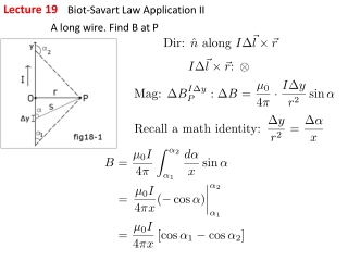
Theory Behind Utility Based Risk Ranking Black Utility Function is for Normal Risk Averse Person Red line is for a Risk Lover Maroon line is for a very risk averse person Blue line is for Risk Neutral Person Utility Income E($) =$5 $10 $0 CE($) Risk Averse DM
Ranking Risky Alternatives Using Utility • Given the assumption: “the DM prefers more to less,” then we can rank risky alternatives with CE • DM will always prefer the risky alternative with the greater CE • To calculate a CE, “all we have to do” is • Assume a utility function • That the DM is rational and consistent, • Calculate DM’s risk aversion coefficient, and • Calculate the DM’s utility for the risky choice • Most of which are impossible!
Ranking Risky Alternatives Using Utility • Utility based risk ranking tools in Simetar • Stochastic dominance with respect to a function (SDRF) • Certainty equivalents (CE) • Stochastic efficiency with respect to a function (SERF) • Risk Premiums (RP) • All of these procedures require estimating the DM’s risk aversion coefficient (RAC) as it is the parameter for the Utility Function • Generally assume a Negative Exponential utility function, so that is easy.
Suggestions on Setting the RACs • Anderson and Dillon (1992) proposed a relative risk aversion (RRAC) schedule of 0.0 risk neutral 0.5 hardly risk averse 1.0 normal or somewhat risk averse 2.0 moderately risk averse 3.0 very risk averse 4.0 extremely risk averse (4.01 is a maximum) • Rule for setting RRAC and ARAC range is:
Estimate the Your Risk Aversion Coefficient (RAC) • Calculate RAC levels for alternative gambles. • Here the gamble is between 0 and 10 • Enter values in the cells that are Yellow to indicate your CE values for the gambles • Lecture 19 Elicit Utility .xlsx
On Assuming a Utility Function for the DM • Power utility function • Use this function when assuming the DM exhibits relative risk aversion RRAC: • DM willing to take on more risk as wealth increases • Poor person buys a $1 lottery ticket • A rich person buys 1,000 $1 lottery tickets • Both may feel the same amount of risk relative to wealth • Use when ranking risky scenarios with a KOV that is calculated over multiple years, as: • Net Present Value (NPV) • Present Value of Ending Net Worth (PVENW)
On Assuming a Utility Function for the DM • Negative Exponential utility function • Use this function when assuming DM exhibits constant absolute risk aversion ARAC • DM will not take on more risk as wealth increases • Poor person buys one $1 lottery ticket • A rich person buys one $1 lottery ticket • Both feel that same amount of risk relative to wealth • Use when ranking risky scenarios using KOVs for a single year, such as: • Annual net cash income or return on investments • NOTE: You get the same rankings with Power and Negative Exponential utility functions, if you use correct the RACs
Four Ranking Risky Methods • First Degree Stochastic Dominance • Second Degree Stochastic Dominance • Generalized Stochastic Dominance with Respect to a (utility) Function • SDRF • Certainty Equivalent CE • Stochastic Efficiency with respect to a Function • SERF • StopLight Charts covered in Lecture 18 are often times more useful for explaining preferences for risky alternatives. Especially if the rankings are supported by SERF
1. Stochastic Dominance • Stochastic Dominance assumes • Decision maker is an expected value maximizer • Risky alternative distributions (F and G) are mutually exclusive. (They are two scenarios we simulated.) • Distributions F(y) and G(y) are based on population probability distributions. In simulation, they are 500 iterations for alternative scenarios of a KOV, e.g. NPV • First degree stochastic dominance when CDFs do not cross • In this case we can say, “All decision makers prefer distribution whose CDF is furthest to the right.” • No need for a utility function in this case, all DMs choose the same risky alternative • However, we are not always lucky enough to have distributions that do not cross.
First Degree Stochastic Dominance • Distribution to the right has higher income at every probability level so it is preferred by all DMs.
---------------------------------------------------------------------------------------------------------------------------------------------------------------------------------------------------------------------------------------------------------------------------------- P(x) F(x) is blue CDF G(x) is red CDF 0.0 A B NPV for F and G Second Degree Stochastic Dominance • SDRF measures the difference between two risky distributions, F and G, at each value on the Y axis • No utility function is used 1.0 • F(x) dominates G(x) for NPV values from zero to A and G(x) dominates from A to B, F(x) dominates for NPV values > B • At each probability, calculate F(x) minus G(x) (the horizontal bars between F and G) and keep track of the net sum of the differences • The net sum of the differences in the end determines which alternative dominates.
---------------------------------------------------------------------------------------------------------------------------------------------------------------------------------------------------------------------------------------------------------------------------------- P(x) F(x) is blue CDF G(x) is red CDF 0.0 A B NPV for F and G Stochastic Dominance wrt a Function (SDRF) or Generalized Stoch. Dominance • SDRF measures the difference between two risky distributions, F and G, at each value on the Y axis, and weights the differences by a utility function using the DM’s ARAC. Assumes a Negative Exponential Utility function in Simetar and Jack Meyer’s original article. 1.0 • F(x) dominates G(x) for NPV values from zero to A and G(x) dominates from A to B, F(x) dominates for NPV values > B • At each probability, calculate F(x) minus G(x) (the horizontal bars between F and G) and weight the difference by a utility function for the upper and lower RACs • Sum the differences and keep score of U(F(x)) <?> U(G(x))
First and Second Degree Stochastic Dominance • In the SDRF worksheet you will find these tables • First Degree says Alt 1 is FDSD over Alt 2 • Second table indicates that Alt 1, Alt 3, Alt 4, and Alt 5 are second degree dominate over Alt 2; and Alt 1 is second degree dominate over Alt 5
Generalized Stochastic Dominance Ranking (SDRF) • Interpretation of a sample Stochastic Dominance result • For all decision makers with a RAC between -0.01 to 0.000287: • The preferred scenario is Alt 4 – the efficient set • Note that Stochastic Dominance resulted in a split decision for the second place rankings • The Lower RAC says Alt 3 is second most preferred while the Risk averse DM prefers Alt 1 second • This is a problem with SDRF that is remedied by SERF
2. Certainty Equivalent (CE) • Compare CE of all risky alternatives at each RAC level • Simetar function for CE is =CERTEQ(range of data, RAC) • Assumes a Negative Exponential Utility Function, but has options for alternative utility functions • Pick the scenario with the largest CE
3. Stochastic Efficiency (SERF) • Stochastic Efficiency with Respect to a Function (SERF) calculates the certainty equivalent for risky alternatives at 25 different RAC levels between the min and max RACs • Compare CE of all risky alternatives at each RAC level • Scenario with the highest CE for the DM’s RAC is the preferred scenario • Summarize the CE results for possible RACs in a chart • Identify the “efficient set” based on the highest CE within a range of RACs • Ranks all scenarios simultaneously • Efficient Set is utility shorthand for saying the risky alternative(s) that is (are) the most preferred
Ranking Scenarios with Stochastic Efficiency (SERF) • SERF requires an assumption about the decision makers’ utility function and like SDRF uses a range of RAC’s • SERF ranks risky strategies based on expected utility which is expressed as CE at the DM’s RAC level • Simetar includes SERF and calculates a table of CE’s over a range of RAC values from the LRAC to the URAC and develops a chart for ranking alternatives
Ranking Scenarios with SERF • SERF results point out why SDRF often produces inconsistent rankings • SDRF only uses the minimum and maximum RACs • The efficient set (ranking) generally differs from the minimum RAC to the maximum RAC • Changing the RACs and re-running SDRF can be slow • SERF can show the actual RAC where the decision maker is indifferent between scenarios where the CE lines cross (this is the BRAC or breakeven risk aversion coefficient) • The SERF Table is best understood as a chart
Ranking Risky Alternatives with SERF • Interpret the SERF chart as follows • The risky alternative that has the highest CE at a particular RAC is the preferred strategy • Within a range of RACs the risky alternative which has the highest CE line is preferred • If the CE lines cross at that point the DM is indifferent between the two risky alternatives and find a BRAC • If the CE line goes negative, the DM would rather earn nothing than to invest in that alternative • Interpret the rankings within risk aversion intervals • RAC = 0 is for risk neutral DM’s • RAC = 1 or 1/W is for normal slightly risk aversion DM’s • RAC = 2 or 2/W is for moderately risk averse DM’s • RAC = 4 or 4/W is for extremely risk averse DM’s
Ranking Scenarios with SERF • Two examples are presented next • The first is for ranking an annual decision using annual net cash income • Uses negative exponential utility function • Lower ARAC = zero • Upper ARAC = 4.00001/Wealth • The second example is for ranking a multiple year decision using NPV variable • Uses Power Utility function • Lower RRAC = zero • Upper RRAC = 4.00001
Additional Considerations for Ranking Risky Alternatives • Advanced materials provided as an appendix • The following overheads are to good to trash but make the lecture to long • They complement Chapter 10 • READ CHAPTER 10!!!
Ranking Risky Alternatives • X=random income simulated for Alter 1 • Y=random income simulated for Alter 2 • Level of income realized for either is x or y • If risk neutral, prefer Alter 1 if E(X) > E(Y) • In terms of utility theory, prefer Alter 1 iff • E(U(X)) > E(U(Y)) • Given that expected utility is calculated as E(U(X)) =∑ [P(X=x) * U(x)] for all levels x where P(X=x) is probability income equals x
Ranking Risky Alternatives • Each risky alternative has a unique CE once we assume a utility function or U(CE) = E(U(X)) • Constant absolute risk aversion (CARA) means that if we add $1 to each outcome we do not change the ranking • If a bet pays $10 or $0 with probability of 50% it may have a CE of $4 • Then if a bet pays $11 or $0 with Probability of 50% the CE is greater than $4 • CARA is a reasonable assumption and it allows us to demonstrate risk ranking
Ranking Risky Alternatives • A CARA utility function is the negative exponential function • U(x) = A - EXP(-x r) • A is a constant to convert income to positives • r is the ARAC or absolute risk aversion coefficient • x is the realized income for the alternative • EXP is the exponent function in Excel • We can estimate the decision maker’s RAC by asking a series of questions regarding gambles
Ranking Risky Alternatives • Calculate Utility for a random return or income given a RAC • U(x) = A – EXP(- (x+scalar) * r) • Let A = 1000 to scale all utility values to positive • Can try different RAC values such as 0.001 Lecture 15
Alternative RACs Lecture 15
Add or Subtract a Constant $ Amount Lecture 15
Ranking Risky Alternatives • Three steps in Utility Analysis • 1st convert the monetary payoffs to utility values using a utility function as U(X) =A-EXP(-x*r) and repeat this step for Y • 2nd calculate the expected value of U(x) as E(U(X)) = ∑ P(X=x) * [A-EXP(-x*r)] Repeat this step for risky alternative Y • 3rd convert the E(U(X)) and the E(U(Y)) to a CE CE(X) > CE(Y) means we prefer X to Y based on the DM ARAC of r and the utility function and the simulated Y and X values • A short cut is to calculate CE directly for a decision makers RAC • Simetar includes a function for calculating CE =CERTEQ(risky income, RAC)
Ranking Risky Alternatives Lecture 15