Download
1 / 22
240 likes | 650 Vues
3.2 Unconstrained Growth. Malthusian Population Model. Thomas Malthus (1766 – 1834). or. Differential equation. The power of population is indefinitely greater than the power in the earth to produce subsistence for man T. Malthus Mathematically:.

E N D
Malthusian Population Model Thomas Malthus (1766 – 1834) or Differential equation The power of population is indefinitely greater than the power in the earth to produce subsistence for man • T. Malthus Mathematically:
Malthusian Population Model (instantaneous, continuous) growth rate; constant of proportionality r = 0.1 Initial condition: P(0) = 100
Finite Difference Equation • In a system-dynamics tool like Vensim (or in a computer program), we simulate continuous time via small, discrete steps. • So instead of using dP/dt for growth, we have DP/Dt: • Then solve for population(t) ….
Finite Difference Equation • In other words: • new_population = old_population + change_in_population • In general, a finite difference equation has the form • new_value = old_value + change_in_value • Such an equation is an approximation to a differential equation (equal in the limit as Dt approaches 0)
Quick Review Question 1 • Consider the differential equation dQ/dt = -0.0004Q, with Q0 = 200. • Using delta notation, give a finite difference equation corresponding to the differential equation. • At time t = 9.0 sec, give the time at the previous time step, where Dt = 0.5 sec. • If Q(t-Dt) = 199.32 and Q(t) = 199.28, give DQ.
Quick Review Question 2 • Evaluate to six decimal places population(.045), the population at the next time interval after the end of Table 3.2.1. Table 3.2.1 Table of Estimated Populations, Where the Initial Population is 100, the Continuous Growth Rate is 10% per Hour, and the Time Step is 0.005 hr ___________________________________________________________________________ tpopulation(t) = population(t-Dt) + (growth) * Dt 0.000 100.000000 0.005 100.050000 = 100.050000 + 10.000000 * 0.005 • Let’s do it in Excel….
Simulation Algorithms: Background • An algorithm is an explicit step-by-step procedure for solving a problem. • Basic building blocks are • Sequencing (one instruction after another) • Conditionals (IF … THEN … ELSE) • Looping (For 100 steps, do the following:) • Assignment statements use left arrows: x x + 1 Al-Khwarizmi (ca. 780-850)
Algorithm 1: Unconstrained Growth initialize simulationLength initialize population initialize growthRate initialize length of time step Dt numIterations simulationLength / Dt for i going from 1 through numIterations do: growth growthRate * population population population + growth*Dt t i*Dt display t, growth, and population
Removing Loop Invariants • If we don’t need to display growth, we can remove the implicit, loop-invariant product growthRate * Dt used to compute population: for i going from 1 through numIterations do: growth growthRate * population population population + growth*Dt t i* Dt display t, growth, and population population population + growthRate*Dt*population
Removing Loop Invariants • Then we save time by computing growthRate * Dt just once, before the loop: initialize simulationLength initialize population initialize growthRate initialize length of time step Dt numIterations simulationLength / Dt growthRatePerStep growthRate * Dt for i going from 1 through numIterations do: population population + growthRatePerStep*population t i*Dt display t and population
Analytical Solutions • Some problems can be solved analytically, without simulation • For example, calculus tells us that the solution to dP/dt = 0.10P with initial condition P0 = 100 is P = 100e0.10t • If such solutions exist, we should use them. But the point of modeling a system is usually that no analytical solution exists.
Analytical Solution via Indefinite Integrals • Separation of variables: move dependent variable (P(t)) and independent variable (t) to opposite sides of equal sign: • Then integrate both sides:
Analytical Solution via Indefinite Integrals • Solve the integral, using e.g. a free online tool like http://integrals.wolfram.com : • Some tools use log for ln • Don’t forget to add constant C • Solve for P using algebra + fact that eln(x) = x
Completion of Analytical Solution • Need constant kin • We know P = 100 at t = 0, so • So analytical solution is
General Solution to Differential Equation for Unconstrained Growth In general, the solution to with initial population P0 is
Quick Review Question 3 • Give the solution to the differential equation where P0 = 57
Unconstrained Decay • For some systems r is negative • E.g., radioactive decay of carbon-14:
Unconstrained Decay half-life (time to decay to half original amount)
Quick Review Question 4 • Radium-226 has a continuous decay rate of about 0.0427869% per year. Determine its half-life in whole years.
Quick Review Question 4 • Radium-226 has a continuous decay rate of about 0.0427869% per year. Determine its half-life in whole years. • Answer: 1620 years