Chapter 3 UNCONSTRAINED OPTIMIZATION

1. Chapter 3 UNCONSTRAINED OPTIMIZATION Prof. S.S. Jang Department of Chemical Engineering National Tsing-Hua Univeristy

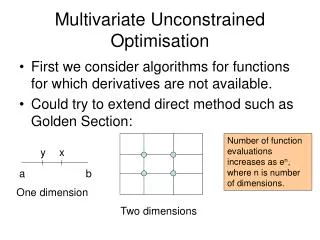
2. Contents • Optimality Criteria • Direct Search Methods • Nelder and Mead (Simplex Search) • Hook and Jeeves(Pattern Search) • Powell’s Method (The Conjugated Direction Search) • Gradient Based Methods • Cauchy’s method (the Steepest Decent) • Newton’s Method • Conjugate Gradient Method (The Fletcher and Reese Method) • Quasi-Newton Method – Variable Metric Method

3. 3-1 The Optimality Criteria • Given a function (objective function) f(x), where and let • Stationary Condition: • Sufficient minimum criteria positive definite • Sufficient maximum criteria negative definite

4. Definiteness • A real quadratic for Q=xTCx and its symmetric matrix C=[cjk] are said to be positive definite (p.d.) if Q>0 for all x≠0. A necessary and sufficient condition for p.d. is that all the determinants: are positive, C is negative definitive (n.d.) if –C is p.d.

5. Example : • x=linspace(-3,3);y=x; • >> for i=1:100 • for j=1:100 • z(i,j)=2*x(i)*x(i)+4*x(i)*y(j)-10*x(i)*y(j)^3+y(j)^2; • end • end • mesh(x,y,z) • contour(x,y,z,100)

6. Example- Continued (mesh and contour)

7. Example-Continued At Indefinite, x* is a non-optimum point.

8. Mesh and Contour – Himmelblau’s function : f(x)=(x12+x2-11)2+(x1+x22-7)2 • Optimality Criteria may find a local minimum in this case • x=linspace(-5,5);y=x; • for i=1:100 • for j=1:100 • z(i,j)=(x(i)^2+y(j)-11)^2+(x(i)+y(j)^2-7)^2; • end • end • mesh(x,y,z) • contour(x,y,z,80)

9. Mesh and Contour - Continued

10. Example: f(x)=x12+25x22

11. Rosenbrock’s Banana Functionf(x,y)=100(y-x2)2+(1-x)2

12. Example: f(x)=2x13+4x1x23-10x1x2+x23Steepest decent search from the initial point at (2,2); we have d=[6x12+4x23-10x2, 12x1x22-10x1+3x22]’=

13. Example: Curve Fitting • From the theoretical considerations, it is believe that the dependent variable y is related to variable x via a two-parameter function: The parameters k1 and k2 are to be determined by a least square of the following experimental data: xy 1.0 1.05 2.0 1.25 3.0 1.55 4.0 1.59

14. Problem Formulation and mesh, contour

15. The Importance of One-dimensional Problem - The Iterative Optimization Procedure Consider a objective function Min f(X)= x12+x22, with an initial point X0=(-4,-1) and a direction (1,0), what is the optimum at this direction, i.e. X1=X0 +*(1,0). This is a one -dimensional search for .

16. 3-2 Steepest Decent Approach – Cauchy’s Method • A direction d=[x1,x2,..,xn]’ is a n-dimensional vector, a line search is an approach such that from a based point x0, find *, for all , x0+ *d is an optimum. • Theorem: the direction d=-[f/x1,f/x2, .., f/xn]’ is the steepest decent direction. Proof: Consider a two dimensional system: f(x1,x2), the movement ds2=dx12+dx22, and f= (f/x1)dx1+ (f/x2)dx2= (f/x1)dx1+ (f/x2)(ds2-dx12)1/2. Then to maximize the change f, we have d(f)/dx1=0. It can be shown that dx1/ds= (f/x1)/((f/x1)2 + (f/x2)2)1/2, dx2/ds= (f/x2)/((f/x1)2+ (f/x2)2)1/2

17. Example: f(x)=2x13+4x1x23-10x1x2+x23Steepest decent search from the initial point at (2,2); we have d=[6x12+4x23-10x2, 12x1x22-10x1+3x22]’=

18. Quadratic Function Properties Property #1: Optimal linear search  for a quadratic function:

19. Quadratic Function Properties- Continued Property #2 fk+1 is orthogonal to sk for a quadratic function

20. 3-2 Newton’s Method – Best Convergence approaching the optimum

21. 3-2 Newton’s Method – Best Convergence approaching the optimum

22. Comparison of Newton’s Method and Cauchy’s Method

23. Remarks • Newton’s method is much more efficient than Steep Decent approach. Especially, the starting point is getting close to the optimum. • There is a requirement for the positive definite of the hessian in implementing Newton’s method. Otherwise, the search will be diverse. • The evaluation of hessian requires second derivative of the objective function, thus, the number of function evaluation will be drastically increased if a numerical derivative is used. • Steepest decent is very inefficient around the optimum, but very efficient at the very beginning of the search.

24. Conclusion • Cauchy’s method is very seldom to use because of its inefficiency around the optimum. • Newton’s method is also very seldom to use because of the requirement of second derivative. • A useful approach should be somewhere in between.

25. 3-3 Method of Powell’s Conjugate Direction • Definition: Let u and v denote two vectors in En. They are said to be orthogonal, if their scalar product equals to zero, i.e. uv=0. Similarly, u and v are said to be mutually conjugative with respect to a matrix A, if u and Av are mutually orthogonal, i.e. uAv=0. • Theorem: If conjugate directions to the hessian are used to any quadratic function of n variables that has a minimum, can be minimized in n steps.

26. Powell’s Conjugated Direction Method-Continued • Corollary: Generation of conjugated vectors-Extended Parallel Space Property • Given a direction d and two initial point x(1), x(2), we assume:

27. Powell’s Algorithm • Step 1: Define x0, and set N linearly indep. Directions say: • s(i)=e(i) • Step 2: Perfrom N+1 one directional searches along with s(N), s(1),,s(N) • Step 3: Form the conjugate direction d using the extended parallel space property. • Step 4: Set • Go to Step 2

28. Powell’s Algorithm (MATLAB) • function opt=powell_n_dim(x0,n,eps,tol,opt_func) • xx=x0;obj_old=feval(opt_func,x0);s=zeros(n,n);obj=obj_old;df=100;absdx=100; • for i=1:n;s(i,i)=1;end • while df>eps/absdx>tol • x_old=xx; • for i=1:n+1 • if(i==n+1) j=1; else j=i; end • ss=s(:,j); • alopt=one_dim_pw(xx,ss',opt_func); • xx=xx+alopt*ss'; • if(i==1) • y1=xx; • end • if(i==n+1) • y2=xx; • end • end • d=y2-y1; • nn=norm(d,'fro'); • for i=1:n • d(i)=d(i)/nn; • end • dd=d'; • alopt=one_dim_pw(xx,dd',opt_func); • xx=xx+alopt*d • dx=xx-x_old; • plot(xx(1),xx(2),'ro') • absdx=norm(dx,'fro'); • obj=feval(opt_func,xx); • df=abs(obj-obj_old); • obj_old=obj; • for i=1:n-1 • s(:,i)=s(:,i+1); • end • s(:,n)=dd; • end • opt=xx

29. Example: f(x)=x12+25x22

30. Example 2: Rosenbrock’s function

31. Example: fittings • x0=[3 3];opt=fminsearch('fittings',x0) • opt = • 2.0884 1.0623

32. Fittings

33. Function Fminsearch • >> help fminsearch • FMINSEARCH Multidimensional unconstrained nonlinear minimization (Nelder-Mead). • X = FMINSEARCH(FUN,X0) starts at X0 and finds a local minimizer X of the • function FUN. FUN accepts input X and returns a scalar function value • F evaluated at X. X0 can be a scalar, vector or matrix. • X = FMINSEARCH(FUN,X0,OPTIONS) minimizes with the default optimization • parameters replaced by values in the structure OPTIONS, created • with the OPTIMSET function. See OPTIMSET for details. FMINSEARCH uses • these options: Display, TolX, TolFun, MaxFunEvals, and MaxIter. • X = FMINSEARCH(FUN,X0,OPTIONS,P1,P2,...) provides for additional • arguments which are passed to the objective function, F=feval(FUN,X,P1,P2,...). • Pass an empty matrix for OPTIONS to use the default values. • (Use OPTIONS = [] as a place holder if no options are set.) • [X,FVAL]= FMINSEARCH(...) returns the value of the objective function, • described in FUN, at X. • [X,FVAL,EXITFLAG] = FMINSEARCH(...) returns a string EXITFLAG that • describes the exit condition of FMINSEARCH. • If EXITFLAG is: • 1 then FMINSEARCH converged with a solution X. • 0 then the maximum number of iterations was reached. • [X,FVAL,EXITFLAG,OUTPUT] = FMINSEARCH(...) returns a structure • OUTPUT with the number of iterations taken in OUTPUT.iterations. • Examples • FUN can be specified using @: • X = fminsearch(@sin,3) • finds a minimum of the SIN function near 3. • In this case, SIN is a function that returns a scalar function value • SIN evaluated at X. • FUN can also be an inline object: • X = fminsearch(inline('norm(x)'),[1;2;3]) • returns a minimum near [0;0;0]. • FMINSEARCH uses the Nelder-Mead simplex (direct search) method. • See also OPTIMSET, FMINBND, @, INLINE.

34. P2 P1 Q … D L Pipeline design

35. 3-4 Conjugated Gradient Method Fletcher-Reeves’s Method (FRP) • Given s1=-f1, s2=-f2+s1 • It can be shown that if • where, s2 is started at the optimum of the line search along the direction s1. And fa+bTxk+1/2xkTHxk, then s2 is conjugated to s1 with respect to H • Most general iteration:

36. Example: (The Fletcher-Reeves Method for Rosenbrock’s function )

37. 3-5 Quasi-Newton’s Method (Variable Matrix Method) • The variable matric approach is using an approximate Hessian matrix without taking second derivative of the objective function, the Newton’s direction can be approximated by: xk+1=xk-kAkfk • As Ak=I Cauchy’s direction • As Ak=H-1 Newton’s direction • In the variable matric approach, Ak can be updated to approximate the inverse of the Hessian by iterative approaches

38. 3-5 Quasi-Newton’s Method (Variable Matrix Method)- Continued • Given the objective function f(x)a+bx+ 1/2xTHx, then f b+Hx, and fk+1- f kH(xk+1- xk ), or xk+1- xk= H-1gk where gk =fk+1- f k • Let Ak+1=H-1 = Ak+ Ak  xk+1- xk= (Ak+ Ak )gk •  Ak gk = xk- Ak gk • Finally,

39. Quasi-Newton’s Method – Continued • Choose y= xk, z= Ak gk (The Davidon-Flecher-Powell’s method • Broyden-Flecher-Shanno’s Method • Summary: • In the first run, given initial conditions and convergence criteria, and evaluate the gradient • First direction is on the negative of the gradient, Ak =I • In the iteration phase, evaluate the new gradient and find gk, xk, and solve Ak using the equation in the previous slide • The new direction is on sk+1=Ak+1f k+1 • Check convergence, and continue the iteration phase

40. Example: (The BFS Method for Rosenbrock’s function )

41. Trial Point Base Point Heuristic Approaches (1) s-2 Simplex Approach • Main Idea • Rules • 1: Straddled: Selected the “worse” vertex generated in the previous iteration, then choose instead the vertex with the next highest function value • 2. Cycling: In a given vertex unchanged more than M iterations, reduce the size by some factor • 3. Termination: The search is terminated when the simlex gets small enough.

42. Example: Rosenbrock Function

43. z xnew xnew xnew xc xc xc X(h) X(h) X(h) xnew z z xc X(h) Simplex Approach: Nelder and Mead xnew

44. Comparisons of Different Approach for Solving Rosenbrock function

45. Heuristic Approach (Reduction Sampling with Random Search) • Step 1: Given initial sampling radius and initial center of the generate a random N points within the region. • Step 2: Get the best of the N sampling as the new center of the circle. • Step 3: Reduce the radius of the search circle, if the radius is not small enough, go back to step 2, otherwise stop.