Download
1 / 30
300 likes | 465 Vues
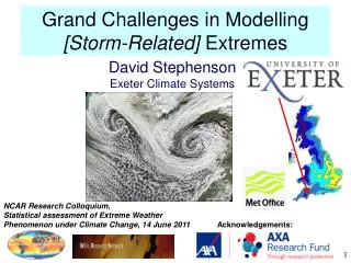
Grand Challenges in Modelling [Storm-Related] Extremes. David Stephenson Exeter Climate Systems. NCAR Research Colloquium, Statistical assessment of Extreme Weather Phenomenon under Climate Change, 14 June 2011. Acknowledgements:. Some grand challenges for climate science.

E N D
Grand Challenges in Modelling [Storm-Related] Extremes David Stephenson Exeter Climate Systems NCAR Research Colloquium, Statistical assessment of Extreme Weather Phenomenon under Climate Change, 14 June 2011 Acknowledgements:
Some grand challenges for climate science • How to quantify the collective risk of extremes? • How to calibrate climate model extremes so that they resemble observed extremes? • How to understand and characterize complex spatio-temporal extremal processes?
Extratropical storms Dec 1989 - Feb 1990 Tracks of maxima in 850mb vorticity Wind speed u Example: Wind speed of 15 m/s and radius of 500 km vorticity of 6x10⁻⁵ /s. • Why use vorticity? • More prominent small-scale features allow earlier detection • Much less sensitive to the background state • Directly linked with low-level winds (through circulation) and precipitation (via vertical motion)
Data: storm tracks in 1950-2003 reanalysis • 355,460 eastward cyclone tracks identified using TRACK software • Extended 6-month winters (1 October - 31 March) • 6 hourly NCAR/NCEP reanalyses from 1950-2003 Stormtracks of Dec 1989-Feb1990 Mean transit counts (per month)
Do extratropical storms cluster? Transits +/-100 of Nova Scotia (45°N, 60°W) Transits +/-100 ofBerlin (52°N,12.5°E) Processes that can lead to clusters: • Random sampling • Rate-varying process (hazard rate varies in time) • Clustered process (one event spawns the next) Yes! Especially over western Europe
Counts of storms passing by London "Not everything that can be counted counts, and not everything that counts can be counted" -- Albert Einstein Blue curve = Poisson GLM trend Grey shading = 95% Conf Int. Red curve = Lowess fit (local polynomial regression) lowess() or loess() in R • Variance of counts is substantially greater than the mean (131%) • Long-term trend has negligible effect on the overdispersion (3%)
Dispersion of monthly counts Units: % Substantial clustering over western Europe. Why?? Mailier, P.J., Stephenson, D.B., Ferro, C.A.T. and Hodges, K.I. (2006): Serial clustering of extratropical cyclones, Monthly Weather Review, 134, pp 2224-2240
Does varying-rate explain the clustering? Poisson regression = number of storms, e.g. monthly counts of windstorms. = time-varying, flow dependent rate. = large-scale teleconnection indices (covariates). GLM maximum likelihood estimation of ß0, ßk
Dependence of storm counts on patterns NAO SCA PEU PNA EAP EA/WR Several patterns are required to capture regional storminess changes! See Seierstad et al. (2007)
Do varying-rates explain the clustering? Units: % under under Residual dispersion after regression on teleconnections Dispersion in counts Clustering in counts is well accounted for by variations in rate related to time variations in teleconnections
Aggregate loss caused by extremesRenato Vitolo, Chris Ferro, Theo Economou, Alasdair Hunter, Ian Cook Intensity/loss 3 2 ... N 1 time Aggregate loss (and many extreme indices) are RANDOM SUMs - the sum of a random number of random values ... Katz, R.W. 2002: Stochastic Modeling of Hurricane Damage J. of Applied Meteorology, Vol 41, 754-762
Variations in London counts and mean intensity Positive association between counts and mean magnitude that is mainly due to interannual variations rather than trends.
Correlation between mean intensity and counts Robust positive correlation over most of northern Europe!
The importance of correlation for aggregate lossSynthetic example: 10000 years simulated from Poisson and LogNormal distributions Correlation 0.02 Mean Y 30.4 200yr Y 169.2 Correlation 0.19 Mean Y 28.6 200yr Y 257.7 200-year loss of 257 much greater than 169 obtained for no correlation!!
Reinsurance actuarial assumptions Counts N XN X1 X2 1. The losses are identically distributed: The distribution of X1,X2,...,XN does not change in time: Pr(Xi>u)=1-F(u) for i=1,2,...,N. 2. The losses are independent of one another: The X1,X2,...,XN are independent of one another: e.g. Pr(X1>u & X2>v)=Pr(X1>u)Pr(X2>v); 3. The losses are independent of the counts: The X1,X2,...,XN are independent of the counts N. ... dynamic background state The assumptions are not valid for weather extremes conditional upon the dynamic state of the system!
Calibration of model extremes Chun Kit Ho, Mat Collins, Simon Brown, Chris Ferro DATA Summertime daily mean air temperatures (15 May -15 Sep) O=Observations 1970-1999 from E-OBS gridded dataset (Haylock et al., 2008) G=HadRM3 standard run for 1970-1999 (25 km horizontal resolution) forced by HadCM3; SRES A1B scenario. G’=Future 30-year time slices from HadRM3 standard run forced by HadCM3; SRES A1B scenario • 2010-2039 • 2040-2069 • 2070-2099 We would like to know how extreme daily temperatures might change in future since they have big impacts on society. e.g. Heat-related mortality in London
London daily summer temperatures G G’ n=30*120=3600 days Black line = sample mean Red line = 99th percentile O’ O ???
Probability density functions O,G O,G,G’ Black line = pdf of obs data 1970-1999 Blue line = pdf of climate data 1970-1999 Red line = pdf of climate data 2070-2099 O O’ ???
Calibration strategies G O O’ G’ O’=B(G’) O’=C(O) How to infer distribution of O’ from distributions of O, G and G’? 1. No calibration Assume O’ and G’ have identical distributions (i.e. perfect model!) i.e. Fo’ =FG’ 2. Bias correction Assume O’=B(G’) where B(.)=Fo-1 (FG(.)) 3. Change factor Assume O’=C(O) where C(.)=FG’-1 (FG(.)) 4. Other e.g. EVT fits to tail and then adjust EVT parameters
Bias correction O’=B(G’) Change factorO’=C(O)
Example: mean warming for London (no shape change) Two approaches give different future mean temperatures!
Effect of calibration on extremesChange in 10-summer level 2040-69 relative to 1970-99 No calibrationTg’ - To Bias correctionLocation, scale & shape Change factorLocation + scale Substantial differences between different predictions!
Summary • Storm-related extremes cluster in time due to dynamic modulation of the rate by large-scale circulation patterns. • Correlation exists between counts and mean intensity of extremes – this has large implications for aggregate losses • Climate model extremes are not statistically distributed like observed extremes and so calibration is required. • Different “rational” calibration strategies lead to substantially different predictions of future mean and extremes! • Change factor transformation G G’ is more linear than bias correction transformation GO • Bias correction of extremes can be validated for present day climate whereas change factor can only be used for future changes. • Much more statistical research is required in this area in order to infer reliable estimates of future weather and climate extremes. We need to develop WELL-SPECIFIED PHYSICALLYINFORMED STATISTICALMODELS of the EXTREMAL PROCESSES Thank you for your attention d.b.stephenson@exeter.ac.uk
References Mailier, P.J., Stephenson, D.B., Ferro, C.A.T. and Hodges, K.I. (2006): Serial clustering of extratropical cyclones, Monthly Weather Review, 134, pp 2224-2240. 21 citations and growing! Seierstad, I.A., Stephenson, D.B., and Kvamsto, N.G. (2007): How useful are teleconnection patterns for explaining variability in extratropical storminess? Tellus A, 59 (2), pp 170–181 Kvamsto, N-G., Song, Y., Seierstad, I., Sorteberg, A. and D.B. Stephenson, 2008: Clustering of cyclones in the ARPEGE general circulation model, Tellus A, Vol. 60, No. 3.), pp. 547-556. Vitolo, R., Stephenson, D.B., Cook, I.M. and Mitchell-Wallace, K. (2009): Serial clustering of intense European storms, Meteorologische Zeitschrift, Vol. 18, No. 4, 411-424.
Statistical methods used in climate science • Extreme indices – sample statistics • Basic extreme value modelling • GEV modelling of block maxima • GPD modelling of excesses above high threshold • Point process model of exceedances • More complex EVT models • Inclusion of explanatory factors (e.g. trend, ENSO, etc.) • Spatial pooling • Max stable processes • Bayesian hierarchical models • + many more • Other stochastic process models
Extreme indices are useful and easy but … Frich indices … Oh really? • They don’t always measure extreme values in the tail of the distribution! • They often confound changes in rate and magnitude • They strongly depend on threshold and so make model comparison difficult • They say nothing about extreme behaviour for rarer extreme events at higher thresholds • They generally don’t involve probability so fail to quantify uncertainty (no inferential model) More informative approach: model the extremal process using statistical models whose parameters are then sufficient to provide complete summaries of all other possible statistics (and can simulate!) See: Katz, R.W. (2010) “Statistics of Extremes in Climate Change”, Climatic Change, 100, 71-76
Furthermore … indices are not METRICS! One should avoid the word “metric” unless the statistic has distance properties! Index, sample/descriptive statistic, or measure is a more sensible name! Oxford English Dictionary: Metric - A binary function of a topological space which gives, for any two points of the space, a value equal to the distance between them, or a value treated as analogous to distance for analysis. Properties of a metric: d(x, y) ≥ 0 d(x, y) = 0 if and only if x = y d(x, y) = d(y, x) d(x, z) ≤ d(x, y) + d(y, z)
Exeter Storm Risk GroupDavid Stephenson, Renato Vitolo, Chris Ferro, Mark HollandAlef Sterk, Theo Economou, Alasdair Hunter, Phil Sansom Key areas of interest and expertise: Mathematical and statistical modelling of extratropical and tropical cyclones and the quantification of risk using concepts from extreme value theory, dynamical systems theory, stochastic processes, etc.