Practical plantwide process control : PID tuning
Practical plantwide process control : PID tuning. Sigurd Skogestad, NTNU. Part 4 : PID tuning. Part 2 (4h). PID controller tuning: It pays off to be systematic ! 1. Obtaining first-order plus delay models Open-loop step response From detailed model (half rule )

Practical plantwide process control : PID tuning
E N D
Presentation Transcript
Practicalplantwideprocesscontrol: PID tuning Sigurd Skogestad, NTNU
Part 4: PID tuning Part 2 (4h). PID controller tuning: It paysoff to be systematic! • 1. Obtaining first-order plusdelaymodels • Open-loop stepresponse • From detailedmodel (half rule) • From closed-loop setpointresponse • 2 . Derivation SIMC PID tuning rules • Controller gain, Integral time, derivative time • 3. Special topics • Integratingprocesses (levelcontrol) • Otherspecialprocesses and examples • When do weneed derivative action? • Near-optimalityof SIMC PID tuning rules • Non PID-control: Is there an advantage in using Smith Predictor? (No) • Examples
Operation: Decision and control layers RTO Min J (economics); MV=y1s cs = y1s CV=y1; MV=y2s MPC y2s PID CV=y2; MV=u u (valves)
Time domain (“ideal” PID) Laplace domain (“ideal”/”parallel” form) For our purposes. Simpler with cascade form Usually τD=0. Then the two forms are identical. Only two parameters left (Kc and τI) How difficult can it be to tune??? Surprisingly difficult without systematic approach! PID controller e
Trans. ASME, 64, 759-768 (Nov. 1942). Comment: Similar to SIMC for integrating process with ¿c=0: Kc = 1/k’ 1/µ ¿I = 4 µ • Disadvantages Ziegler-Nichols: • Aggressive settings • No tuning parameter • Poor for processes with large time delay (µ)
Disadvantage IMC-PID (=Lambda tuning): Many rules Poor disturbance response for «slow» processes (with large ¿1/µ)
Motivation for developing SIMC PID tuning rules • The tuning rules should be well motivated, and preferably be model-based and analytically derived. • They should be simple and easy to memorize. • They should work well on a wide range of processes.
SIMC PI tuning rule • Approximate process as first-order with delay (e.g., use “half rule”) • k = process gain • ¿1 = process time constant • µ = process delay • Derive SIMC tuning rule*: Open-loop step response c¸ -: Desired closed-loop response time (tuning parameter) Integral time rule combines well-known rules: IMC (Lamda-tuning): Same as SIMC for small ¿1 (¿I = ¿1) Ziegler-Nichols: Similar to SIMC for large ¿1 (if we choose ¿c= 0; aggressive!) Reference: S. Skogestad, “Simple analytic rules for model reduction and PID controller design”, J.Proc.Control, Vol. 13, 291-309, 2003 (*) “Probably the best simple PID tuning rules in the world”
Model: Dynamic effect of change in input u (MV) on output y (CV) First-order + delay model for PI-control Second-order model for PID-control Recommend: Use second-order model only if ¿2>µ MODEL Need a model for tuning
MODEL, Approach 1A 1. Step response experiment • Make step change in one u (MV) at a time • Record the output (s) y (CV)
MODEL, Approach 1A Δy(∞) RESULTING OUTPUT y STEP IN INPUT u Δu : Delay - Time where output does not change 1: Time constant - Additional time to reach 63% of final change k = y(∞)/ u : Steady-state gain
MODEL, Approach 1A Step response integrating process Δy Δt
MODEL, Approach 1B Shams’ method: Closed-loop setpoint response with P-controller with about 20-40% overshoot Kc0=1.5 Δys=1 Δy∞ • OBTAIN DATA IN RED (first overshoot • and undershoot), and then: • tp=4.4, dyp=0.79; dyu=0.54, Kc0=1.5, dys=1 • dyinf = 0.45*(dyp + dyu) • Mo =(dyp -dyinf)/dyinf % Mo=overshoot (about 0.3) • b=dyinf/dys • A = 1.152*Mo^2 - 1.607*Mo + 1.0 • r = 2*A*abs(b/(1-b)) • %2. OBTAIN FIRST-ORDER MODEL: • k = (1/Kc0) * abs(b/(1-b)) • theta = tp*[0.309 + 0.209*exp(-0.61*r)] • tau = theta*r • 3. CAN THEN USE SIMC PI-rule Δyp=0.79 Δyu=0.54 tp=4.4 Example 2: Get k=0.99, theta =1.68, tau=3.03 Ref: Shamssuzzoha and Skogestad (JPC, 2010) + modification by C. Grimholt (Project, NTNU, 2010; see also PID-book 2012)
Start with complicated stable model on the form Want to get a simplified model on the form Most important parameter is the “effective” delay MODEL, Approach 2 2. Model reduction of more complicated model
MODEL, Approach 2 Example 1 Half rule
MODEL, Approach 2 original 1st-order+delay
MODEL, Approach 2 2 half rule
MODEL, Approach 2 original 1st-order+delay 2nd-order+delay
MODEL, Approach 2 c c c c c c Approximation of zeros To make these rules more general (and not only applicable to the choice c=): Replace (time delay) by c (desired closed-loop response time). (6 places) Alternative and improvedmethodforfapproximating zeros: Simple Analytic PID Controller Tuning Rules Revisited J Lee, W Cho, TF Edgar - Industrial & Engineering Chemistry Research 2014, 53 (13), pp5038–5047
PI-controller (based on first-order model) For second-order model add D-action. For our purposes, simplest with the “series” (cascade) PID-form: SIMC-tunings Derivation of SIMC-PID tuning rules
SIMC-tunings Basis: Direct synthesis (IMC) Closed-loop response to setpoint change Idea: Specify desired response: and from this get the controller. ……. Algebra:
SIMC-tunings NOTE: Setting the steady-state gain = 1 in T will result in integral action in the controller!
SIMC-tunings IMC Tuning = Direct Synthesis Algebra:
SIMC-tunings d u y c g Integral time • Found: Integral time = dominant time constant (I = 1) (IMC-rule) • Works well for setpoint changes • Needs to be modified (reduced) for integrating disturbances Example. “Almost-integrating process” with disturbance at input: G(s) = e-s/(30s+1) Original integral time I = 30 gives poor disturbance response Try reducing it!
SIMC-tunings I = 1 Reduce I to this value: I = 4 (c+) = 8 Integral Time Setpoint change at t=0 Input disturbance at t=20
SIMC-tunings Integral time • Want to reduce the integral time for “integrating” processes, but to avoid “slow oscillations” we must require: • Derivation: • Setpoint response: Improve (get rid of overshoot) by “pre-filtering”, y’s = f(s) ys. Details: See www.nt.ntnu.no/users/skoge/publications/2003/tuningPID Remark 13 II
SIMC-tunings Conclusion: SIMC-PID Tuning Rules One tuning parameter: c
SIMC-tunings Some insights from tuning rules • The effective delay θ (which limits the achievable closed-loop time constant τc) is independent of the dominant process time constant τ1! • It depends on τ2/2 (PI) or τ3/2 (PID) • Use (close to) P-control for integrating process • Beware of large I-action (small τI) for level control • Use (close to) I-control for fast process (with small time constant τ1) • Parameter variations: For robustness tune at operating point with maximum value of k’θ = (k/τ1)θ
SIMC-tunings Selection of tuning parameter c Two main cases • TIGHT CONTROL: Want “fastest possible control” subject to having good robustness • Want tight control of active constraints (“squeeze and shift”) • SMOOTH CONTROL: Want “slowest possible control” subject to acceptable disturbance rejection • Want smooth control if fast setpoint tracking is not required, for example, levels and unconstrained (“self-optimizing”) variables • THERE ARE ALSO OTHER ISSUES: Input saturation etc. TIGHT CONTROL: SMOOTH CONTROL:
TIGHT CONTROL Typical closed-loop SIMC responses with the choice c=
TIGHT CONTROL Example. Integrating process with delay=1. G(s) = e-s/s. Model: k’=1, =1, 1=1 SIMC-tunings with c with ==1: IMC has I=1 Ziegler-Nichols is usually a bit aggressive Setpoint change at t=0c Input disturbance at t=20
TIGHT CONTROL • Approximate as first-order model with k=1, 1 = 1+0.1=1.1, =0.1+0.04+0.008 = 0.148 • Get SIMC PI-tunings (c=): Kc = 1 ¢ 1.1/(2¢ 0.148) = 3.71, I=min(1.1,8¢ 0.148) = 1.1 2. Approximate as second-order model with k=1, 1 = 1, 2=0.2+0.02=0.22, =0.02+0.008 = 0.028 Get SIMC PID-tunings (c=): Kc = 1 ¢ 1/(2¢ 0.028) = 17.9, I=min(1,8¢ 0.028) = 0.224, D=0.22
SMOOTH CONTROL Will derive Kc,min. From this we can get c,max using SIMC tuning rule Tuning for smooth control • Tuning parameter: c = desired closed-loop response time • Selecting c=(“tight control”) is reasonable for cases with a relatively large effective delay • Other cases: Select c > for • slower control • smoother input usage • less disturbing effect on rest of the plant • less sensitivity to measurement noise • better robustness • Question: Given that we require some disturbance rejection. • What is the largest possible value for c ? • Or equivalently: The smallest possible value for Kc? S. Skogestad, ``Tuning for smooth PID control with acceptable disturbance rejection'', Ind.Eng.Chem.Res, 45 (23), 7817-7822 (2006).
SMOOTH CONTROL Closed-loop disturbance rejection d0 -d0 ymax -ymax
Kc u SMOOTH CONTROL Minimum controller gain for PI-and PID-control: min |c(j)| = Kc
SMOOTH CONTROL Rule: Min. controller gain for acceptable disturbance rejection:Kc¸ |ud|/|ymax| often ~1 (in span-scaled variables) |ymax| = allowed deviation for output (CV) |ud| = required change in input (MV) for disturbance rejection (steady state) = observed change (movement) in input from historical data
SMOOTH CONTROL Rule: Kc¸ |ud|/|ymax| • Exception to rule: Can have lower Kc if disturbances are handled by the integral action. • Disturbances must occur at a frequency lower than 1/I • Applies to: Process with short time constant (1 is small) and no delay (¼ 0). • For example, flow control • Then I = 1 is small so integral action is “large”
SMOOTH CONTROL Summary: Tuning of easy loops • Easy loops: Small effective delay (¼ 0), so closed-loop response time c (>> ) is selected for “smooth control” • ASSUME VARIABLES HAVE BEEN SCALED WITH RESPECT TO THEIR SPAN SO THAT |u0/ymax| = 1 (approx.). • Flow control: Kc=0.2, I = 1 = time constant valve (typically, 2 to 10s; close to pure integrating!) • Level control: Kc=2 (and no integral action) • Other easy loops (e.g. pressure): Kc = 2, I = min(4c, 1) • Note: Often want a tight pressure control loop (so may have Kc=10 or larger)
3. Derivative time: Only for dominant second-order processes Conclusion PID tuning
PID: More (Special topics) • Integrating processes (level control) • Other special processes and examples • When do we need derivative action? • Near-optimality of SIMC PID tuning rules • Non PID-control: Is there an advantage in using Smith Predictor? (No) KFUPM-Distillation Control Course
SMOOTH CONTROL LEVEL CONTROL q LC V 1. Application of smooth control • Averaging level control If you insist on integral action then this value avoids cycling Reason for having tank is to smoothen disturbances in concentration and flow. Tight level control is not desired: gives no “smoothening” of flow disturbances. Proof: 1. Let |u0| = |q0| – expected flow change [m3/s] (input disturbance) |ymax| = |Vmax| - largest allowed variation in level [m3] Minimum controller gain for acceptable disturbance rejection: Kc¸ Kc,min = |u0|/|ymax| = |q0| / |Vmax| 2. From the material balance (dV/dt = q – qout), the model is g(s)=k’/s with k’=1. Select Kc=Kc,min. SIMC-Integral time for integrating process: I = 4 / (k’ Kc) = 4 |Vmax| / | q0| = 4 ¢ residence time provided tank is nominally half full and q0 is equal to the nominal flow.
LEVEL CONTROL More on level control • Level control often causes problems • Typical story: • Level loop starts oscillating • Operator detunes by decreasing controller gain • Level loop oscillates even more • ...... • ??? • Explanation: Level is by itself unstable and requires control.
LEVEL CONTROL Level control: Can have both fast and slow oscillations • Slow oscillations (Kc too low): P > 3¿I • Fast oscillations (Kc too high): P < 3¿I Here: Consider the less common slow oscillations
LEVEL CONTROL How avoid oscillating levels? 0.1 ¼ 1/2
LEVEL CONTROL Case study oscillating level • We were called upon to solve a problem with oscillations in a distillation column • Closer analysis: Problem was oscillating reboiler level in upstream column • Use of Sigurd’s rule solved the problem