ENE 429 Antenna and Transmission lines Theory

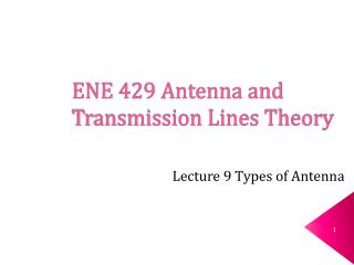
1. DATE: 24/07/06 28/07/06 ENE 429Antenna and Transmission lines Theory Lecture 4 Transmission lines

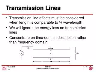
2. Transmission lines (1) • Transmission lines or T-lines are used to guide propagation of EM waves at high frequencies. • Examples: • Transmitter and antenna • Connections between computers in a network • Interconnects between components of a stereo system • Connection between a cable service provider and aTV set. • Connection between devices on circuit board • Distances between devices are separated by much larger order of wavelength than those in the normal electrical circuits causing time delay.

3. Transmission lines (2) • Properties to address: • time delay • reflections • attenuation • distortion

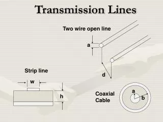
4. Distributed-parameter model • Types of transmission lines

5. Distributed-parameter model • The differential segment of the transmission line R’ = resistance per unit length L’= inductance per unit length C’= capacitor per unit length G’= conductance per unit length

6. Telegraphist’s equations • General transmission lines equations:

7. Telegraphist’s time-harmonic wave equations • Time-harmonic waves on transmission lines After arranging we have where

8. Traveling wave equations for the transmission line • Instantaneous form • Phasor form

9. Lossless transmission line • lossless when R’ = 0 and G’ = 0 and

10. Low loss transmission line (1) • low loss when R’ << L’ and G’ << C’ Expanding in binomial series gives for x << 1

11. Low loss transmission line (2) Therefore, we get

12. Characteristic impedance • Characteristic impedance Z0is defined as the the ratio of the traveling voltage wave amplitude to the traveling current wave amplitude. or For lossless line,

13. Power transmission • Power transmitted over a specific distance is calculated. • The instantaneous power in the +z traveling wave at any point along the transmission line can be shown as • The time-averaged power can be shown as W.

14. Power ratios on the decibel scale (1) • A convenient way to measure power ratios • Power gain (dB) • Power loss (dB) • 1 Np = 8.686 dB dB dB

15. Power ratios on the decibel scale (2) • Representation of absolute power levels is the dBm scale dBm

16. Ex1 A 12-dB amplifier is in series with a 4-dB attenuator. What is the overall gain of the circuit?Ex2 If 1 W of power is inserted into a coaxial cable, and 1 W of power is measured 100m down the line, what is the line’s attenuation in dB/m?

17. Ex3 A 20 m length of the transmission line is known to produce a 2 dB drop in the power from end to end, • what fraction of the input power does it reach the output? • What fraction of the input power does it reach the midpoint of the line? • What is the attenuation constant?

18. Wave reflection at discontinuities • To satisfy boundary conditions between two dissimilar lines • If the line is lossy, Z0will be complex.

19. Reflection coefficient at the load (1) • The phasor voltage along the line can be shown as • The phasor voltage and current at the load is the sum of incident and reflected values evaluated at z = 0.

20. Reflection coefficient at the load (2) • Reflection coefficient • A reflected wave will experience a reduction in amplitude and a phase shift • Transmission coefficient

21. Power transmission in terms of reflection coefficient W W W

22. Total power transmission (matched condition) • The main objective in transmitting power to a load is to configure line/load combination such that there is no reflection, that means.

23. Voltage standing wave ratio • Incident and reflected waves create “Standing wave”. • Knowing standing waves or the voltage amplitude as a function of position helps determine load and input impedances Voltage standing wave ratio

24. Forms of voltage (1) • If a load is matched then no reflected wave occurs, the voltage will be the same at every point. • If the load is terminated in short or open circuit, the total voltage form becomes a standing wave. • If the reflected voltage is neither 0 nor 100 percent of the incident voltage then the total voltage will compose of both traveling and standing waves.

25. Forms of voltage (2) • let a load be position at z = 0 and the input wave amplitude is V0, where

26. Forms of voltage (3) we can show that traveling wave standing wave • The maximum amplitude occurs when • The minimum amplitude occurs when standing waves become null,

27. The locations where minimum and maximum voltage amplitudes occur (1) • The minimum voltage amplitude occurs when two phase terms have a phase difference of odd multiples of . • The maximum voltage amplitude occurs when two phase terms are the same or have a phase difference of even multiples of .

28. The locations where minimum and maximum voltage amplitudes occur (2) • If  = 0,  is real and positive and • zmin and zmaxare separated by multiples of one-half wavelength. The distance between zmin and zmax is a quarter wavelength. • We can show that

29. Ex4 Slotted line measurements yield a VSWR of 5, a 15 cm between successive voltage maximum, and the first maximum is at a distance of 7.5 cm in front of the load. Determine load impedance, assuming Z0 = 50 .