Transmission Lines
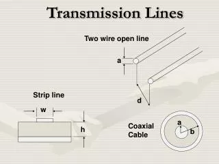
Transmission Lines. Transmission Lines. Cross-sectional view of typical transmission lines (a) coaxial line, (b) two-wire line, (c) planar line, (d) wire above conducting plane, (e) microstrip line.

Transmission Lines
E N D
Presentation Transcript
Transmission Lines
Transmission Lines Cross-sectional view of typical transmission lines (a) coaxial line, (b) two-wire line, (c) planar line, (d) wire above conducting plane, (e) microstrip line. (a) Coaxial line connecting the generator to the load; (b) E and H fields on the coaxial line
Transmission Lines Electric and magnetic fields around single-phase transmission line Triplate line Stray field
Transmission Lines Transmission LinesTransmission Line Equations for a Lossless Line The transmission line consists of two parallel and uniform conuductors, not necessarily identical. Where L and C are the inductance and capacitance per unit length of the line, respectively.
Transmission Lines iNS (N+1)’ N’ Definitions of currents and voltages for the lumped-circuit transmission-line model. By applying Kirchhoff’s voltage law to N - (N + 1) - (N + 1)’ - N’ loop, we obtain If node N is at the position z, node (N +1) is at position z + h, and
Transmission Lines Since h is an arbitrary small distance, we can let h approach zero Applying Kirchhoff’s current law to node N we get from which
Transmission Lines All cross-sectional information about the particular line is contained in L and C Telegrapher’s Equations Wave Equation
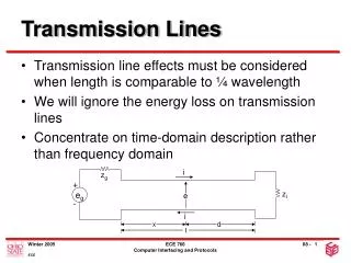
Transmission Lines Waves on the Lossless Transmission Line Roughly speaking, a wave is a disturbance that moves away from its source as time passes. Suppose that the voltage on a transmission line as a function of position z and time t has the form V(z,t) = f(z-Ut)U = const This is the same function as f(z), but shifted to the right a distance of Ut along the z axis. The displacement increases as time increases. The velocity of motion is U. x = Z-Ut f(x) has its maximum where x = z – Ut = 0, and the position of maximum Zmaxat t = tois given by Zmax= Uto Any function of the argument (z-Ut) keeps its shape and moves as a unit in the +z direction. For example, let f(x) be the triangular function shown in (a). Then at time t=0 f(z-Ut)=f(z) is the function of z shown in (b). At a later time to , f(z-Ut)=f(z-Uto) is the function of z shown in (c). Note that the pulse is moving to the right with velocity U.
Transmission Lines The function V(z,t) = f(z-Ut) describes undistorted propogation in the +z direction and represents a solution of the wave equation for a lossless transmission line: Wave Equation The wave equation is satisfied provided that The leftward-traveling wave v(z,t) = f(z+Ut) is also a solution.
v(z,t)=Acos(kz-ωt) (U= ω/k) Transmission Lines t = 0 An important special case is that in which the function f is a sinusoid. Fig (a) shows the function v(z,t)=Acos(kz-ωt) as it appears if photographed with a flash camera at time t=0. In (b) it is seen at the later time to t = to The wavelength of the wave is defined as the distance between the maxima at any fixed instant of time. V(z,t) has maxima when its argument (kz-ωt) is zero, ±2π, ±4π, etc. At t = 0, there is a maximum at z = 0. The next one occurs when kz = 2π, or z = 2π / k. λ= 2π / k U = 2πf / k = λf
Transmission Lines The separation of time and space dependence for sinusoidal (time – harmonic) waves is achieved by the use of phasors. Phasors are the complex quantities (in polar form) representing the magnitude and the phase of sinusoidal functions. Phasors are independent of time. Time-harmonic function expressed as a cosine wave Time Factor “The real part of” Phasor For a wave moving in the +z direction, The phasor representing this positive – going wave is For a wave moving to the left,
Transmission Lines A = const at all z since we are dealing with a lossless line. However, the phase does vary with z. For the leftward – moving wave, the phasor would rotate in the counter – clockwise direction. Right-ward moving wave
Transmission Lines Characteristic Impedance The positive - going voltage wave: (A=constant, Φ = constant) Instantaneous voltage Voltage phasor The second telegrapher’s equation in phasor form For the positive – going wave, Characteristic impedance (independent of position) Since and - real number (50-400Ω)
Transmission Lines Characteristic Impedance continued For a negative – going wave, Power transmitted by a single wave (average power; the instantaneous power oscillates at twice the fundamental frequency)
Transmission Lines Reflection and Transmission At z = 0, Assuming that the incident wave is known and solving for , we obtain Load’s Reflection Coefficient
Transmission Lines Reflection and Transmission continued Example Suppose ZL = ∞ (open circuit). Find the distribution of the voltage on the line if the incident wave is Assume that A is real (Φ= 0) The total voltage on the line is: at The instantaneous voltage is: at all times. At The total voltage is the sum of the two waves of equal amplitude moving in opposite directions. The positions of zero total voltage stand still. This phenomenon is referred to as a standing wave. In the case of a single traveling wave, , there are positions where the voltage vanishes, but these positions move at the velocity of the wave
Transmission Lines Reflection and Transmission continued If (short circuit), and Again we have a standing wave but with the nulls at If (resistive), When n=1 ( , i.e. the line is terminated in its characteristic impedance), the reflected wave vanishes Suppose that one more transmission line is connected at the load terminals (z=0) Z02 Z01
Transmission Lines Reflection and Transmission continued The voltage at z=0, if we approach from the left, is . If we . Thus we can write: approach from the right, it is Applying Kirchhoff’s current law we get Further, , , and , The currents and can be expressed in term of , ,respectively: and Now, assuming that is known, we can find (Transmission Coefficient) (Reflection Coefficient)
Transmission Lines Standing-Wave Ratio (losseless transmission line) The total phasor voltage as a function of position on a line connected to a load at z=0 is The magnitude of the reflected voltage phasor is The amplitude of voltage as a function of z At any position, the instantaneous voltage on the line is a sinusoidal function of time, with the amplitude given by the above expression. The amplitude regularly increases and decreases as the cosine function varies. The positions of voltage amplitude maxima and minima are stationary (independent of time). This phenomenon is referred to as a standing wave.
Transmission Lines Standing-Wave Ratio continued (losseless transmission line) In the special case of , the reflected wave vanishes and there is only a single traveling wave moving to the right. In this case the voltage amplitude is independent of position (“flat” voltage profile). If there are two (or more) traveling waves on the line, they will interact to produce a standing wave.
Transmission Lines Standing-Wave Ratio continued (losseless transmission line) an integer The standing-wave ratio (SWR) is defined as SWR = 1 when For two adjacent maxima at, say, N=1 and N=0 we can write Voltage maxima and minima repeat every half wavelength.
Transmission Lines Transmission Line Equations for a Lossy Line (sinusoidal waves) From Kirchhoff’s laws in their phasor form, we have Proceeding as before (for a lossless lines), we obtain the phasor form of the telegrapher equations, where L, R, C, and G are, respectively, the series inductance, series resistance, shunt capacitance, and shunt conductance per unit length. The corresponding (voltage) wave equation is The two solutions of the wave equation are +z -z where and are constants describing the wave’s amplitude and phase and is the propagation constant.
Transmission Lines Transmission Line Equations for a Lossy Line continued (sinusoidal waves) The propagation constant of a lossy transmission line is (complex number) where and are real numbers. Inserting R=0, G=0 (lossless line) we obtain For the positive-going wave Causes negative phase shift (phasor rotates clockwise as z increases) Causes attenuation (amplitude becomes smaller exponentially as z increases)
Transmission Lines Transmission Line Equations for a Lossy Line continued (sinusoidal waves) A phase shift of equal to corresponds to the wave travel distance z equal to the wavelength : is the phase constant (measured in radians per meter) is the attenuation constant (measured in Nepers per meter) is the attenuation length (amplitude decreases 1/e over z= ) The corresponding instantaneous voltage is In general, nonlinear functions of ω (A is assumed to be real) The position of a maximum is given by As t increases, the maximum moves to the right with velocity - Phase Velocity (Up)
Transmission Lines Dispersion In general, the phase velocity Upis a function of frequency; that is, a signal containing many frequencies tends to become ‘dispersed’ (some parts of the signal arrived sooner and others later.) Up is independent of frequency for (1) lossless lines (R=0, G=0) and (2) distortionless lines (R/L=G/C) because for those lines βis a linear function of ω. Cut-off frequency Example of dispersion diagram for an arbitrary system that is characterized by Up>c Upat any frequency is equal to the slope of a line drawn from the origin to the corresponding point on the graph. For ω= radians/second Up = ∞. In general, Up can be either greater or less then c. Information in a wave travels at a different velocity known as the group velocity is equal to the slope of the tangent to the ω-βcurve at the frequency in question (for for this particular system). always remains less then c.
Transmission Lines Non-Sinusoidal Waves (lossless transmission line) Reflection of a rectangular pulse of a short circuit. (a) Shows the incident pulse moving to the right. In (b) it is striking the short-circuit termination, note that the sum of the incident and the reflected voltages must always be zero at that position. In (c) the reflected pulse is moving to the left.
Transmission Lines Multiple Reflections +z -z +z t1 t2 V0 Example Suppose t2 = ∞ (an infinitely long pulse or a step function) and , so that . Find the total voltage on the line after a very long time. The initial (incident) wave moving to the right has amplitude The first reflected wave moving to the left has amplitude where
Transmission Lines Multiple Reflections continued The second reflected wave moving to the right has amplitude and so on The total voltage at is given by the infinite series Inserting the values of and we find that (simply results from the voltage divider of Rs and RL, as if the line were not there.
Transmission Lines Lattice (bounce) diagram This is a space/time diagram which is used to keep track of multiple reflections. Ideal voltage source z z Voltage at the receiving end
Transmission Lines Points to Remember • In this chapter we have surveyed several different types of waves on transmission lines. It is important that these different cases not be confused. When approaching a transmission-line problem, the student should begin by asking, “Are the waves in this problem sinusoidal, or rectangular pulses? Is the line ideal, or does it have losses?” Then the proper approach to the problem can be taken. • The ideal lossless line supports waves of any shape (sinusoidal or non-sinusoidal), and transmits them without distortion. The velocity of these waves is . The ratio of the voltage to current is , provided that only one wave is present. Sinusoidal waves are treated using phasor analysis. (A common error is that of attempting to analyze non-sinusoidal waves with phasors. Beware! This makes no sense at all.) • When the line contains series resistance and or shunt conductance it is said to be lossy. Lossy lines no longer exhibit undistorted propagation; hence a rectangular pulse launched on such a line will not remain rectangular, instead evolving into irregular, messy shapes. However, sinusoidal waves, because of their unique mathematical properties, do continue to be sinusoidal on lossy lines. The presence of losses changes the velocity of propagation and causes the wave to be attenuated (become smaller) as it travels.
Transmission Lines Points to Remember continued • For lines other than the simple ideal lossless lines, the velocity of propagation usually is a function of frequency. This velocity, the speed of voltage maxima on the line, is properly called the phase velocity Up. The change of Up with frequency is called dispersion. The velocity with which information travels on the line is not Up, but a different velocity, known as the group velocity . The phase velocity is given by . However • 5. Examples of non-sinusoidal waves are short rectangular pulses, and also infinitely long rectangular pulses, which are the same as step functions. Problems involving sudden voltage steps differ from sinusoidal problems, just as in ordinary circuits, problems involving transients differ from the sinusoidal steady state. Pulse problems are usually approached by superposition; that is, one tracks the pulses that propagate back and forth, adding up the waves to obtain the total voltage at any place and time.
Transmission Lines Points to Remember continued • All kinds of waves are reflected at discontinuities in the line. If the line continues beyond the discontinuity, a portion of the wave is transmitted as well. The reflected and transmitted waves are described by the reflection coefficient and the transmission coefficient. For sinusoidal waves there is a simple formula giving the reflection coefficient for any load impedance ZL. For non-sinusoidal waves, the same formula can be used, but only if the load impedance is purely resistive. Otherwise the reflected wave has a different shape from the incident wave, and a reflection coefficient cannot be meaningfully defined. • 7. In the case of non-sinusoidal waves, it is sometimes necessary to add up the contributions of many reflected waves bouncing back and forth on the line. However, for sinusoidal steady-state problems, it is only necessary to consider two waves, one moving to the right and the other to the left. (Lossless line) (Bounce diagram)
Transmission Lines Points to Remember continued • When both an incident and reflected wave are simultaneously present on a transmission line, a standing wave is said to be present. This means that a stationary pattern of voltage maxima and minima is present. The ratio of the maximum voltage to the minimum voltage is called the standing-wave ratio (SWR). The positions of the voltage maxima are determined by the phase angle of the load’s reflection coefficient, and the spacing between each pair of adjacent maxima is λ/2 (and not λ, as one might think). Positions of maximum voltage are positions of minimum current, and vice versa. • 9. The impedance Z(z) at any point on a line is defined as the ratio of the total voltage phasor to the total current phasor at the point z. If a standing wave is present, the impedance will be a periodic function of position along the line, with period λ/2. Note that this impedance is different from the “characteristic impedance” Zo, which is a constant that depends only on the construction of the line. (Sinusoidal Waves) (Sinusoidal Waves)