Download
1 / 53
530 likes | 767 Vues
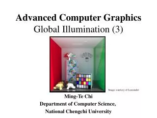
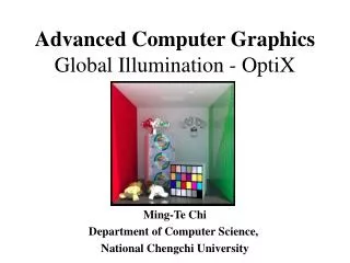
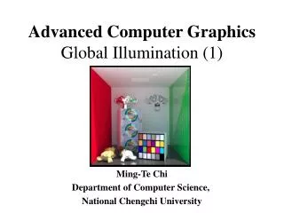
Advanced Computer Graphics Global Illumination (1). Ming-Te Chi Department of Computer Science, National Chengchi University. Global Illumination. Rendering equation Ray tracing Radisoity Photon mapping. Rendering Equation (Kajiya 1986). Consider a point on a surface. N.

E N D
Advanced Computer Graphics Global Illumination (1) • Ming-Te Chi • Department of Computer Science, • National Chengchi University
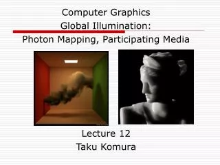
Global Illumination • Rendering equation • Ray tracing • Radisoity • Photon mapping
Rendering Equation (Kajiya 1986) • Consider a point on a surface N Iin(Φin) Iout(Φout)
Rendering Equation • Outgoing light is from two sources • Emission • Reflection of incoming light • Must integrate over all incoming light • Integrate over hemisphere • Must account for foreshortening of incoming light
Rendering Equation Iout(Φout) = E(Φout) + ∫ 2πRbd(Φout, Φin )Iin(Φin) cos θ dω emission angle between Normal and Φin bidirectional reflection coefficient Note that angle is really two angles in 3D and wavelength is fixed
Rendering Equation • Rendering equation is an energy balance • Energy in = energy out • Integrate over hemisphere • Fredholm integral equation • Cannot be solved analytically in general • Various approximations of Rbd give standard rendering models • Should also add an occlusion term in front of right side to account for other objects blocking light from reaching surface
Another version Consider light at a point p arriving from p’ i(p, p’) = υ(p, p’)(ε(p,p’)+ ∫ρ(p, p’, p’’)i(p’, p’’)dp’’) emission from p’ to p occlusion = 0 or attenuation =1/d2 light reflected at p’ from all points p’’ towards p
BRDF database • http://www.merl.com/brdf/
Ray Tracing Slide Courtesy of Roger Crawfis, Ohio State
Ray Tracing • Follow rays of light from a point source • Can account for reflection and transmission
Computation • Should be able to handle all physical interactions • Ray tracing paradigm is not computational • Most rays do not affect what we see • Scattering produces many (infinite) additional rays • Alternative: ray casting
Ray Casting • Only rays that reach the eye matter • Reverse direction and cast rays • Need at least one ray per pixel
Ray Casting Quadrics • Ray casting has become the standard way to visualize quadrics which are implicit surfaces in CSG systems • Constructive Solid Geometry • Primitives are solids • Build objects with set operations • Union, intersection, set difference
Constructive solid geometry (CSG) • Union • intersection • difference
Ray Casting a Sphere • Ray is parametric • Sphere is quadric • Resulting equation is a scalar quadratic equation which gives entry and exit points of ray (or no solution if ray misses)
Shadow Rays • Even if a point is visible, it will not be lit unless we can see a light source from that point • Cast shadow or feeler rays
Reflection • Must follow shadow rays off reflecting or transmitting surfaces • Process is recursive
Computing a Reflected Ray N S S Rout Rin Ɵ Ɵ
Scene with no reflection rays Scene with one layer of reflection Scene with two layer of reflection
Transformed ray d θ N θ r t
Fresnel Reflectance • Fresnel equation describe the behaviour of light when moving between media of differing refractive indices. conductive materials aluminum dielectric glasses
Schlick's approximation the specular reflection coefficient R
Diffuse Surfaces • Theoretically the scattering at each point of intersection generates an infinite number of new rays that should be traced • In practice, we only trace the transmitted and reflected rays, but use the Phong model to compute shade at point of intersection • Radiosity works best for perfectly diffuse (Lambertian) surfaces
Building a Ray Tracer • Best expressed recursively • Can remove recursion later • Image based approach • For each ray ……. • Find intersection with closest surface • Need whole object database available • Complexity of calculation limits object types • Compute lighting at surface • Trace reflected and transmitted rays
When to stop • Some light will be absorbed at each intersection • Track amount left • Ignore rays that go off to infinity • Put large sphere around problem • Count steps
Recursive Ray Tracer(1/3) color c = trace(point p, vector d, int step) { color local, reflected, transmitted; point q; normal n; if(step > max) return(background_color); p d
Recursive Ray Tracer (2/3) N p r q = intersect(p, d, status); if(status==light_source) return(light_source_color); if(status==no_intersection) return(background_color); n = normal(q); r = reflect(q, n); t = transmit(q,n); d q t
Recursive Ray Tracer (3/3) local = phong(q, n, r); reflected = trace(q, r, step+1); transmitted = trace(q,t, step+1); return(local + reflected + transmitted); } N p r d q t
Computing Intersections • Implicit Objects • Quadrics • Planes • Polyhedra • Parametric Surfaces
Implicit Surfaces Ray fromp0in directiond p(t) = p0 +t d General implicit surface f(p) = 0 Solve scalar equation f(p(t)) = 0 General case requires numerical methods
Planes p• n + c = 0 p(t) = p0 +t d t = -(p0• n + c)/ d• n
Quadrics General quadric can be written as pTAp + bTp +c = 0 Substitute equation of ray p(t) = p0 +t d to get quadratic equation Ellipsoid Elliptic paraboloid Hyperbolic paraboloid …..
Polyhedra • Generally we want to intersect with closed objects such as polygons and polyhedra rather than planes • Hence we have to worry about inside/outside testing • For convex objects such as polyhedra there are some fast tests
Ray Tracing Polyhedra • If ray enters an object, it must enter a front facing polygon and leave a back facing polygon • Polyhedron is formed by intersection of planes • Ray enters at furthest intersection with front facing planes • Ray leaves at closest intersection with back facing planes • If entry is further away than exit, ray must miss the polyhedron
Shadows • Ray tracing casts shadow feelers to a point light source. • Many light sources are illuminated over a finite area. • The shadows between these are substantially different. • Area light sources cast soft shadows • Penumbra • Umbra
Soft Shadows Slide Courtesy of Roger Crawfis, Ohio State
Soft Shadows Penumbra Umbra Slide Courtesy of Roger Crawfis, Ohio State
Camera Models • Up to now, we have used a pinhole camera model. • These has everything in focus throughout the scene. • The eye and most cameras have a larger lens or aperature. Slide Courtesy of Roger Crawfis, Ohio State
Motion Blur Slide Courtesy of Roger Crawfis, Ohio State
Supersampling 1 sample per pixel 16 sample per pixel 256 sample per pixel Slide Courtesy of Roger Crawfis, Ohio State