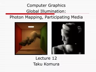
Advances in Global Illumination Techniques for Realistic Rendering
This comprehensive overview discusses global illumination methods in computer graphics, emphasizing key concepts like the rendering equation, ray tracing, radiosity, and photon mapping. It explores the intricacies of light behavior, including emission, reflection, and how these are modeled within the rendering equation. The text delves into practical applications such as ray casting and its importance for visualizing implicit surfaces within Constructive Solid Geometry (CSG). Finally, it covers the recursive nature of ray tracing and strategies for efficient light calculation in complex scenes.

Advances in Global Illumination Techniques for Realistic Rendering
E N D
Presentation Transcript
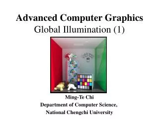
Computer Graphics Global Illumination • 紀明德 mtchi@cs.nccu.edu.tw • Department of Computer Science, • National Chengchi University
Global Illumination • Rendering equation • Ray tracing • Radisoity • Photon mapping
Rendering Equation (Kajiya 1986) • Consider a point on a surface N Iin(Φin) Iout(Φout)
Rendering Equation • Outgoing light is from two sources • Emission • Reflection of incoming light • Must integrate over all incoming light • Integrate over hemisphere • Must account for foreshortening of incoming light
Rendering Equation Iout(Φout) = E(Φout) + ∫ 2πRbd(Φout, Φin )Iin(Φin) cos θ dω emission angle between Normal and Φin bidirectional reflection coefficient Note that angle is really two angles in 3D and wavelength is fixed
Rendering Equation • Rendering equation is an energy balance • Energy in = energy out • Integrate over hemisphere • Fredholm integral equation • Cannot be solved analytically in general • Various approximations of Rbd give standard rendering models • Should also add an occlusion term in front of right side to account for other objects blocking light from reaching surface
Another version Consider light at a point p arriving from p’ i(p, p’) = υ(p, p’)(ε(p,p’)+ ∫ρ(p, p’, p’’)i(p’, p’’)dp’’ emission from p’ to p occlusion = 0 or 1/d2 light reflected at p’ from all points p’’ towards p
RAY TRACING Slide Courtesy of Roger Crawfis, Ohio State
Ray Tracing • Follow rays of light from a point source • Can account for reflection and transmission
Computation • Should be able to handle all physical interactions • Ray tracing paradigm is not computational • Most rays do not affect what we see • Scattering produces many (infinite) additional rays • Alternative: ray casting
Ray Casting • Only rays that reach the eye matter • Reverse direction and cast rays • Need at least one ray per pixel
Ray Casting Quadrics • Ray casting has become the standard way to visualize quadrics which are implicit surfaces in CSG systems • Constructive Solid Geometry • Primitives are solids • Build objects with set operations • Union, intersection, set difference
Ray Casting a Sphere • Ray is parametric • Sphere is quadric • Resulting equation is a scalar quadratic equation which gives entry and exit points of ray (or no solution if ray misses)
Shadow Rays • Even if a point is visible, it will not be lit unless we can see a light source from that point • Cast shadow or feeler rays
Reflection • Must follow shadow rays off reflecting or transmitting surfaces • Process is recursive
Diffuse Surfaces • Theoretically the scattering at each point of intersection generates an infinite number of new rays that should be traced • In practice, we only trace the transmitted and reflected rays, but use the Phong model to compute shade at point of intersection • Radiosity works best for perfectly diffuse (Lambertian) surfaces
Building a Ray Tracer • Best expressed recursively • Can remove recursion later • Image based approach • For each ray ……. • Find intersection with closest surface • Need whole object database available • Complexity of calculation limits object types • Compute lighting at surface • Trace reflected and transmitted rays
When to stop • Some light will be absorbed at each intersection • Track amount left • Ignore rays that go off to infinity • Put large sphere around problem • Count steps
Recursive Ray Tracer(1/3) color c = trace(point p, vector d, int step) { color local, reflected, transmitted; point q; normal n; if(step > max) return(background_color); p d
Recursive Ray Tracer (2/3) N p r q = intersect(p, d, status); if(status==light_source) return(light_source_color); if(status==no_intersection) return(background_color); n = normal(q); r = reflect(q, n); t = transmit(q,n); d q t
Recursive Ray Tracer (3/3) local = phong(q, n, r); reflected = trace(q, r, step+1); transmitted = trace(q,t, step+1); return(local + reflected + transmitted); } N p r d q t
Computing Intersections • Implicit Objects • Quadrics • Planes • Polyhedra • Parametric Surfaces
Implicit Surfaces Ray fromp0in directiond p(t) = p0 +t d General implicit surface f(p) = 0 Solve scalar equation f(p(t)) = 0 General case requires numerical methods
Planes p• n + c = 0 p(t) = p0 +t d t = -(p0• n + c)/ d• n
Polyhedra • Generally we want to intersect with closed objects such as polygons and polyhedra rather than planes • Hence we have to worry about inside/outside testing • For convex objects such as polyhedra there are some fast tests
Ray Tracing Polyhedra • If ray enters an object, it must enter a front facing polygon and leave a back facing polygon • Polyhedron is formed by intersection of planes • Ray enters at furthest intersection with front facing planes • Ray leaves at closest intersection with back facing planes • If entry is further away than exit, ray must miss the polyhedron
RADISOITY courtesy of Cornell
Radiosity • Consider objects to be broken up into flat patches (which may correspond to the polygons in the model) • Assume that patches are perfectly diffuse reflectors • Radiosity = flux = energy/unit area/ unit time leaving patch
Notation n patches numbered 1 to n bi = radiosity of patch I ai = area patch I total intensity leaving patch i = bi ai ei ai = emitted intensity from patch I ρi = reflectivity of patch I fij = form factor = fraction of energy leaving patch j that reaches patch i
Radiosity Equation energy balance biai = eiai + ρi ∑ fjibjaj reciprocity fijai= fjiaj radiosity equation bi = ei + ρi ∑ fijbj
1st pass 2ed pass 3rd pass 4th pass 16th pass
Computing Form Factors • Consider two flat patches
Using Differential Patches foreshortening
Form Factor Integral fij = (1/ai) ∫ai ∫ai (oij cos θi cos θj / πr2 )dai daj occlusion foreshortening of patch j foreshortening of patch i
Solving the Intergral • There are very few cases where the integral has a (simple) closed form solution • Occlusion further complicates solution • Alternative is to use numerical methods • Two step process similar to texture mapping • Hemisphere • Hemicube
Hemisphere • Use illuminating hemisphere • Center hemisphere on patch with normal pointing up • Must shift hemisphere for each point on patch
Hemicube • Easier to use a hemicube instead of a hemisphere • Rule each side into “pixels” • Easier to project on pixels which give delta form factors that can be added up to give desired from factor • To get a delta form factor we need only cast a ray through each pixel