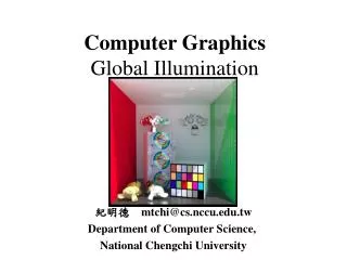
Global Illumination
Global Illumination. CSE167: Computer Graphics Instructor: Steve Rotenberg UCSD, Fall 2005. Classic Ray Tracing. The ‘classic’ ray tracing algorithm shoots one primary ray per pixel

Global Illumination
E N D
Presentation Transcript
Global Illumination CSE167: Computer Graphics Instructor: Steve Rotenberg UCSD, Fall 2005
Classic Ray Tracing • The ‘classic’ ray tracing algorithm shoots one primary ray per pixel • If the ray hits a colored surface, then a shadow ray is shot towards each light source to test for shadows, and determine if the light can contribute to the illumination of the surface • If the ray hits a shiny reflective surface, a secondary ray is spawned in the reflection direction and recursively traced through the scene • If a ray hits a transparent surface, then a reflection and a transmission (refraction) ray are spawned and recursively traced through the scene • To prevent infinite loops, the recursion depth is usually capped to some reasonable number of bounces (less than 10 usually works) • In this way, we may end up with an average of fewer than 20 or so rays per pixel in scenes with only a few lights and a few reflective or refractive surfaces • Scenes with many lights and many inter-reflecting surfaces will require more rays • Images rendered with the classic ray tracing algorithm can contain shadows, exact inter-reflections and refractions, and multiple lights, but may tend to have a rather ‘sharp’ appearance, due to the limitation to perfectly polished surfaces and point light sources
etc. Classic Ray Tracing
Distribution Ray Tracing • Distribution ray tracing extends the classic ray tracing algorithm by shooting several rays in situations where the classic algorithm shoots only one (or two) • For example, if we shoot several primary rays for a single pixel, we can achieve image antialiasing • We can model area light sources, and achieve soft edge shadows by shooting several shadow rays distributed across the light surface • We can model blurry reflections and refractions by spawning several rays distributed around the reflection/refraction direction • We can also model camera focus blur by distributing our rays across a virtual camera aperture • As if that weren’t enough, we can also render motion blur by distributing our primary rays in time • Distribution ray tracing is a powerful extension to classic ray tracing that clearly showed that the central concept of ray tracing was a useful paradigm for high quality rendering • However, it is, of course, much more expensive, as the average number of rays per pixel can jump to hundreds, or even thousands…
etc. etc. Distribution Ray Tracing
Ray Tracing • The classic and distribution ray tracing algorithms are clearly important steps in the direction of photoreal rendering • However, they are not truly physically correct as they still are leaving out some components of the illumination • In particular, they don’t fully sample the hemisphere of possible directions for incoming light reflected off of other surfaces • This leaves out important lighting features such as color bleeding also known as diffuse inter-reflection (for example, if we have a white light source and a diffuse green wall next to a diffuse white wall, the white wall will appear greenish near the green wall, due to green light diffusely reflected off of the green wall) • It also leaves out complex specular effects like focused beams of light known as caustics (like the wavy lines of light seen at the bottom of a swimming pool)
Hemispherical Sampling • We can modify the distribution ray tracing algorithm to shoot a bunch of rays scattered about the hemisphere to capture additional incoming light • With some careful tuning, we can make this operate in a physically plausible way • However, we would need to shoot a lot of rays to adequately sample the entire hemisphere, and each of those rays would have to spawn lots of other rays when they hit surfaces • 10 rays is definitely not enough to sample a hemisphere, but let’s just assume for now that we will use 10 samples for each hemisphere • If we have 2 lights and we supersample the pixel with 16 samples and allow 5 bounces where each bounce shoots 10 rays, we end up with potentially 16*(2+1)*105 = 4,800,000 rays traced to color a single pixel • This makes this approach pretty impractical • The good news is that there are better options…
Path Tracing • In 1985, James Kajiya proposed the Monte Carlo path tracing algorithm, also known as MCPT or simply path tracing • The path tracing algorithm fixes many of the exponential ray problems we get with distribution ray tracing • It assumes that as long as we are taking enough samples of the pixel in total, we shouldn’t have to spawn many rays at each bounce • Instead, we can even get away with spawning a single ray for each bounce, where the ray is randomly scattered somewhere across the hemisphere • For example, to render a single pixel, we may start by shooting 16 primary rays to achieve our pixel antialiasing • For each of those samples, we might only spawn off, say 10 new rays, scattered in random directions • From then on, any additional bounces will spawn off only 1 new ray, thus creating a path. In this example, we would be tracing a total of 16*10 paths per pixel • We will still end up shooting more than 160 rays, however, as each path may have several bounces and will also spawn off shadow rays at each bounce • Therefore, if we allow 5 bounces and 2 lights, as in the last example, we will have a total of (2+1)*(5+1) = 18 rays per path, for a total of 8*160=1280 rays per pixel, which is a lot, but far more reasonable than the previous example
BRDFs • In a previous lecture, we briefly introduced the concept of a BRDF, or bidirectional reflectance distribution function • The BRDF is a function that describes how light is scattered (reflected) off of a surface • The BRDF can model the macroscopic behavior of microscopic surface features such as roughness, different pigments, fine scale structure, and more • The BRDF can provide everything necessary to determine how much light from an incident beam coming from any direction will scatter off in any other direction • Different BRDFs have been designed to model the complex light scattering patterns from a wide range of materials including brushed metals, human skin, car paint, glass, CDs, and more • BRDFs can also be measured from real world materials using specialized equipment
BRDF Formulation • The wavelength dependent BRDF at a point is a 5D function BRDF = fr(θi,φi,θr,φr,λ) • Often, instead of thinking of it as a 5D scalar function of λ, we can think of it as a 4D function that returns a color BRDF = fr(θi,φi,θr,φr) • Another option is to express it in more of a vector notation: BRDF = fr(ωi,ωr) • Sometimes, it is also expressed as a function of position: BRDF = fr(x,ωi,ωr)
Physically Plausible BRDFs • For a BRDF to be physically plausible, it must not violate two key laws of physics: • Helmholtz reciprocity fr(ωi,ωr) = fr(ωr,ωi) Helmholtz reciprocity refers to the reversibility of light paths. We should be able to reverse the incident and reflected ray directions and get the same result. It is this important property of light that makes algorithms like ray tracing possible, as they rely on tracing light paths backwards • Conservation of energy ∫Ωfr(ωi,ωr)(ωr·n)dωr < 1, for all ωi For a BRDF to conserve energy, it must not reflect more light than it receives. A single beam of incident light may be scattered across the entire hemisphere above the surface. The total amount of this reflected light is the (double) integral of the BRDF over the hemisphere of possible reflection directions
BRDF Evaluation • The outgoing radiance along a vector ωr due to an incoming radiance (irradiance) from direction ωi: dLr(x,ωr)=fr(x,ωi,ωr)Li(x,ωi)(ωi·n)dωi • To compute the total outgoing radiance along vector ωr, we must integrate over the hemisphere of incoming radiance: Lr(x,ωr)=∫Ωfr(x,ωi,ωr)Li(x,ωi)(ωi·n)dωi
Rendering Equation Lr(x,ωr)=∫Ωfr(x,ωi,ωr)Li(x,ωi)(ωi·n)dωi • This equation is known as the rendering equation, and is the key mathematical equation behind modern photoreal rendering • It describes the light Lrreflected off from some location x in some direction ωr • For example, if our primary ray hits some surface, we want to know the light reflected off of that point back in the direction towards the camera • The reflected light is described as an integral over a hemispherical domain Ω, which is really just shorthand for writing it as a double integral over two angular variables • We integrate over the hemisphere of possible incident light directions ωi • Given a particular incident light direction ωi and our desired reflection direction ωr, we evaluate the BRDF fr() at location x • The BRDF tells us how much the light coming from direction ωi will be scaled, but we still need to know how much light is coming from that direction. Unfortunately, this involves computing Li(), which involves solving an integral equation exactly like the one we’re already trying to solve • The rendering equation is unfortunately, an infinitely recursive integral equation, which makes it rather difficult to compute
Monte Carlo Sampling • Path tracing is based on a mathematical concept of Monte Carlo sampling • Monte Carlo sampling refers to algorithms that make use of randomness to compute a mathematical result (Monte Carlo famous for its casinos) • Technically, we use Monte Carlo sampling to approximate a complex integral that we can’t solve analytically • For example, consider computing the area of a circle. Now, we have a simple analytical formula for that, but we can apply Monte Carlo sampling to it anyway • We consider a square area around our circle and choose a bunch of random points distributed in the square. If we count the number of points that end up inside the circle, we can approximate the area of the circle as: (area of square) * (number of points in circle) / (total number of points) • Monte Carlo sampling is a ‘brute force’ computation method for approximating complex integrals that can’t be solved with any other reasonable way. It is often considered as a last resort to solving complex problems, as it can at least try to approximate any integral equation, but it may require lots of samples
Limitations of Path Tracing • Path tracing can be used to render any lighting effect, but might require many paths to adequately resolve complex situations • Some situations are simply too complex for the algorithm and would require too many paths to make it practical • It is particularly bad at capturing specularly bounced light and focused beams of light • Path tracing will converge on the ‘correct’ solution, given enough paths, so it can be used to generate reference images of how a scene should look. This can be useful for evaluating and comparing with other techniques
Bidirectional Path Tracing • Bidirectional path tracing (BPT) is an extension to the basic path tracing algorithm that attempts to handle indirect light paths better • For each pixel, several bidirectional paths are examined • We start by tracing a ray path from the eye as in path tracing. We then shoot a photon path out from one of the light sources • Lets say each path has 5 rays in it and 5 intersection points • We then connect each of the intersection points in the eye path with each of the intersection points in the light path with a new ray • If the ray is unblocked, we add a contribution of the new path that connects from the light source to the eye • The BPT algorithm improves on path tracing’s ability to handle indirect light (such as a room lit by light fixtures that shine on the ceiling)
Metropolis Sampling • Metropolis sampling is another variation of a path tracing type algorithm • For some pixel, we start by tracing a path from the eye to some light source • We then make a series of random ‘modifications’ to the path and test the amount of light from that path • Based on a statistical algorithm that uses randomness, a decision is made whether or not to ‘keep’ the new path or discard it • Whichever way is chosen, the resulting path is then modified again and the algorithm is repeated • Metropolis sampling is quite a bizarre algorithm and makes use of some complex properties of statistics • It tends to be good at rendering highly bounced light paths such as a room lit by skylight coming through a window, or the caustic light patterns one sees at the bottom of swimming pools • The Metropolis algorithm is difficult to implement and requires some very heuristic components • It has demonstrated an ability to render features that very few other techniques can handle, although it has not gained wide acceptance and tends to be limited to academic research
Photon Mapping • In 1995, Henrik Jensen proposed the photon mapping algorithm • Photon mapping starts by shooting many (millions) of photons from the light sources in the scene, scattered in random directions • Each photon may bounce off of several surfaces in a direction that is random, but biased by the BRDF of the surface • For each hit, a statistical (random) decision is made whether or not the photon will bounce or ‘stick’ in the surface, eventually leading to all photons sticking somewhere • The photons are collected into a 3D data structure (like a KD tree) and stored as a bunch of 3D points with some additional information (color, direction…) • Next, the scene is rendered with a ray/path tracing type approach • Rays are shot from the camera and may spawn new rays off of sharp reflecting or refracting surfaces • The more diffuse components of the lighting can come from analyzing the photon map • To compute the local lighting due to photons, we collect all of the photons within some radius of our sample point • The photons we collect are used to contribute to the lighting of that point
Photon Mapping • There are many variations on the photon mapping algorithm and there are different ways to use the photon map • The technique can also be combined with other approaches like path tracing • Photon mapping tends to be particularly good at rendering caustics, which had previously been very difficult • As the photon mapping algorithm stores the photons as simple points in space, the photon map itself is independent of the scene geometry, making the algorithm very flexible and able to work with any type of geometry • Some of the early pictures of photon mapping showed focused caustics through a glass of sherry, shining onto a surface of procedurally generated sand- a task that would have been impossible with any previous technique
Volumetric Photon Mapping • A later extension to the core photon mapping algorithm allowed interactions between photons and volumetric objects like smoke • A photon traveling through a participating media like smoke will travel in a straight line until it happens to hit a smoke particle, then it will scatter in some random direction, based on the scattering function of the media • This can be implemented by randomly determining the point at which the photon hits a particle (or determining that it doesn’t hit a anything, allowing it to pass through) • As with surfaces, the photons will also be able to ‘stick’ in the volume • Volumetric photon mapping allows accurate rendering of beams of light (even beams of reflected or focused light) to properly scatter through smoke and fog, with the scattered light properly illuminating other objects nearby
Translucency • The photon mapping algorithm (and other ray based rendering algorithms) has also been adapted to trace the paths of photons scattered through translucent surfaces
Local vs. Global Illumination • High quality photoreal rendering requires two key things: • Accurate modeling of light interactions with materials (local illumination) • Accurate modeling of light bouncing around within an environment (global illumination) • The local illumination is modeled with the use of BRDFs. Various BRDF functions have been designed to model the appearance of a variety of materials. BRDFs can also be scanned from real-world objects • The global illumination is computed by tracing light paths in the environment. The various ray-based algorithms take different approaches to evaluating the paths