Light, Reflectance, and Global Illumination

Light, Reflectance,and Global Illumination • TOPICS: • Survey of Representations for Light and Visibility • Color, Perception, and Light • Reflectance • Cost of Ray Tracing • Global Illumination Overview • Radiosity • Yu’s Inverse Global Illumination paper • 15-869, Image-Based Modeling and Rendering • Paul Heckbert, 18 Oct. 1999

Representations for Light and Visibility

Physics of Light and Color • Light comes from electromagnetic radiation. • The amplitude of radiation is a function of wavelength . • Any quantity related to wavelength is called “spectral”. • Frequency  = 2  /  • EM spectrum: • radio, infrared, visible, ultraviolet, x-ray, gamma-ray • long wavelength short wavelength • low frequency high frequency • Don’t confuse EM ``spectrum’’ with ``spectrum’’ of signal in signal/image processing; they’re usually conceptually distinct. • Likewise, don’t confuse spectral wavelength & frequency of EM spectrum with spatial wavelength & frequency in image processing.

Perception of Light and Color • Light is electromagnetic radiation visible to the human eye. • Humans have evolved to sense the dominant wavelengths emitted by the sun; space aliens have presumably evolved differently. • In low light, we perceive primarily with rods in the retina, which have broad spectral sensitivity (“at night, you can’t see color”). • In bright light, we perceive primarily with the three sets of cones in the retina, which have narrower spectral sensitivity roughly corresponding to red, yellow, and blue wavelengths. • We’re most sensitive to greens & yellows; not very sens. to blue. • The eye has a huge dynamic range: 10 orders of magnitude. • In the brain, neurons combine cone signals into spot, edge, and line receptive fields (point spread functions). And each comes at a range of scales, orientations, and color channels.

What is Color? • Color is human perception of light. • Our perception is imperfect; we don’t see spectral power P(), instead we see three scalars: • at long wavelength ( red): L = P()sL()d • at middle wavelength ( yellow): M = P()sM()d • at short wavelength ( blue): S = P()sS()d • where sL(), sM(), and sS() are the sensitivity curves of our three sets of cones. • Color is three dimensional because any light we see is indistinguishable to our eyes from some mixture of three spectral (monochromatic, single-wavelength) primaries.

Color Spaces • Color can be described in various color spaces: • spectrum - allows non-visible radiation to be described, but usually impractical/unnecessary. • RGB - CRT-oriented color space • good for computer storage. • HSV - a more intuitive color space; good for user interfaces • H=hue -- the color wheel, the spectral colors • S=saturation (purity) -- how gray? • V=value (related to brightness, luminance) -- how bright? • a non-linear transform of RGB, since H is cyclic. • CIE XYZ - used by color scientists, a linear transform of RGB. • other color spaces, less commonly used... • For extremely realistic image synthesis, use of four or more samples of the spectrum may be necessary, but for most purposes, the three samples used by RGB color space is just fine.

Light is a Function of Many Variables • Light is a function of • position x,y,z • direction  • wavelength  • time t • polarization • phase • In computer graphics, we typically ignore the last three by assuming static scenes, unpolarized, incoherent light, and assume that the speed of light is infinite. • But light is still a complicated function of many variables. • How do we measure light, what are the units?

Units of Light • quantity dimension units • solid angle solid angle [steradian] • power energy/time [watt]=[joule/sec] • radiance L power/(area*solid angle) [watt/(m2*steradian)] • a.k.a. intensity I • In vacuum or as an approximation for air, radiance is constant along a ray. • A picture is an array of incoming radiance values at imaginary projection plane; because of radiance-constancy, these are equal to outgoing radiances at intersection of ray with first surface hit • In general, light is absorbed and scattered along a ray.

General Reflection & Transmission • At a surface, reflectance is the fraction of incident (incoming) light that is reflected, transmittance is the fraction that is transmitted into the material. Opaque materials have zero transmittance. • In some books, reflectance is denoted , and transmittance . Other books use kdr and ksr for diffuse and specular reflectance, and kdt and kst for transmittance. • A general reflectance function has the form of a bidirectional reflectance distribution function (BRDF): (i,i,o,o), where the direction of incoming light is (i,i) and the direction of outgoing light is (o,o),  is the polar angle measured from perpendicular, and  is the azimuth. • There is a similar function for bidirectional transmittance, (i,i,o,o). • Light is absorbed and scattered by some media (e.g. fog). • Phong’s Illumination model is an approximation to general reflectance.

Phong Illumination Model • A point light source with radiance Il, illuminating an opaque surface, reflects light of the following radiance: • If surface is perfectly diffuse (Lambertian). It is independent of viewing direction! • I = Il kdr max{N.L,0}/r2 • where kdr = coefficient of diffuse reflection [1/steradian] • N = unit normal vector • L = unit direction vector to light, r is distance to light • If surface is perfectly specular. It is not independent of viewing direction. • I = Il ksr max{N.H,0}e/r2 • where ksr = coefficient of specular reflection [1/steradian] • H = unit “halfway vector” = (V+L)/||V+L|| • V = unit direction vector to viewer • e = exponent, controlling apparent roughness: small=rough, big=smooth • There are more realistic reflection models than Phong’s. • Don’t confuse Phong Illumination with Phong Shading.

Cost of Basic Rendering Algorithms • s = #surfaces (e.g. polygons) ts = time per surface (transforming, ...) • p = #pixels tp = time per pixel (writing, incrementing, ...) •  = #lights t = time to light surface point w.r.t. one light • a =  screen areas of surfs ti = time for one ray/surface intersection test • Painter’s or Z-buffer algorithm, with flat shading • (assuming no sorting in painter’s algorithm) • worst case cost = s(ts+ t) + atpatp if polygons big • Painter’s or Z-buffer algorithm, with per pixel shading (e.g. Phong) • worst case cost = sts+ a(t+ tp) atif polygons big • Ray casting with no shadows, no spatial data structures • worst case cost = p(sti+ t + tp) pstiif many surfaces • Ray tracing to max depth d with shadows, refl&tran, no spat. DS, no supersampling • 2d1 intersections/pixel, for each of which there are  shadow rays • worst case cost = p(2d1)[( +1)sti+ t] 2dpstiif many surfaces • Note: time constants vary, e.g. tp is larger for z-buffer than for painter’s.

Interreflection • We typically simulate just direct illumination: light traveling on a straight, unoccluded line from light source to surface, reflected there, then traveling in a straight, unoccluded line into eye. • Light travels by a variety of paths: • light source  eye (0 bounces: looking at light source) • light source  surface1  eye (1 bounce: direct illumination) • light source  surf1  surf2  eye (2 bounces) • light source  surf1  surf2  surf3  eye (3 bounces) • ... • Illumination via a path of 2 or more bounces is called indirect illumination or interreflection. It also happens with transmission.

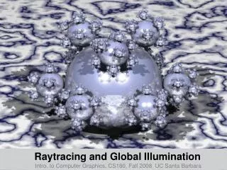
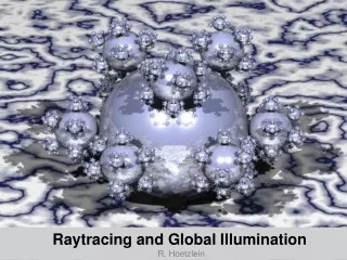
Global Illumination • Observation: light comes from other surfaces, not just designated light sources. • Goal: simulate interreflection of light in 3-D scenes. • Difficulty: you can no longer shade surfaces one at a time, since they’re now interrelated! • Two general classes of algorithms: • 1. ray tracing methods: simulate motion of photons one by one, tracing photon paths either backwards (“eye ray tracing”) or forwards (“light ray tracing”) -- good for specular scenes • 2. radiosity methods: set up a system of linear equations whose solution is the light distribution -- good for diffuse scenes

The Unit of Radiosity • Radiance (a.k.a. intensity) is power from/to an area in a given direction. • units: power / (area  solid angle) • Radiosity is outgoing power per unit area due to emission or reflection over a hemisphere of directions. • units: power / area • radiosity = radiance  integral of [cos(polar angle)  d(solid angle)] over a hemisphere =  radiance • So radiosity and radiance are linearly interrelated. • Thus, “radiosity” is both a unit of light and an algorithm. • Radiant emitted flux density is the unit for light emission. • units: power / area

Radiosity as an Integral Equation • This is called an integral equation because the unknown function “radiosity(x)” appears inside an integral. • Can be solved by radiosity methods or randomized “Monte Carlo” techniques also, by simulating millions of photon paths. • Radiosity methods are a discrete way to think about and simulate global illumination. where x and t are surface points

Classical Radiosity Method • Definitions: • surfaces are divided into elements • radiosity = integral of emitted radiance plus reflected radiance over a hemisphere. units: [power/area] • Assumptions: • no participating media (no fog) shade surfaces only, not vols. • opaque surfaces (no transmission) • reflection and emission are diffuse radiance is direction-indep., radiance is a function of 2-D surface parameters and  • reflection and emission are independent of  within each of several wavelength bands; typically use 3 bands: R,G,B solve 3 linear systems of equations • radiosity is constant across each element one RGB radiosity per element • Typically (but not exclusively): • surfaces are polygons, elements are quadrilaterals or triangles

Deriving Radiosity Equations, 1

Form Factors • Define the form factorFij to be the fraction of light leaving element i that arrives at element j • Where • vij is a boolean visibility function: 0 if point on i is occluded with respect to point on j, 1 if unoccluded. • This is a double area integral. Difficult! We end up approximating it. • dAi and dAj are infinitesimal areas on elements i and j, respectively • i and j are polar angles: the angles between ray and normals on elements i and j, respectively • Projected area of dAi from j is cos idAi, hence the cosines • r is distance from point on i to point on j • Reciprocity law: AiFij = AjFji.

Deriving Radiosity Equations, 2

Computing Visibility for Form Factors • Computing visibility in the form factor integral is like solving a hidden surface problem from the point of view of each surface in the scene. • Two methods: • ray tracing: easy to implement, but can be slow without spatial subdivision methods (grids, octrees, hierarchical bounding volumes) to speed up ray-surface intersection testing • hemicube: exploit speed of z-buffer algorithm, compute visibility between one element and all other elements. Good when you have z-buffer hardware, but some tricky issues regarding hemicube resolution • You end up approximating the double area integral with a double summation, just like numerical methods for approximating integrals. • When two elements are known to be inter-visible (no occluders), you can use analytic form factor formulas and skip all this.

Radiosity Systems Issues • All algorithms require the following operations: • 1. Input scene (geometry, emissions, reflectances). • 2. Choose mesh (important!), subdividing polygons into elements. • 3. Compute form factors using ray tracing or hemicube for visibility (expensive). • 4. Solve system of equations (indirectly, if progressive radiosity). • 5. Display picture. • If mesh is chosen too coarse, approximation is poor, you get blocky shadows. • If mesh is chosen too fine, algorithm is slow. A good mesh is critical! • In radiosity simulations, because scene is assumed diffuse, surfaces’ radiance will be view-independent. • Changes in viewpoint require only visibility computations, not shading. Do with z-buffer hardware for speed. This is commonly used for “architectural walkthroughs” and virtual reality. • Changes in scene geometry or reflectance require a new radiosity simulation.

Summary of Radiosity Algorithms • Radiosity algorithms allow indirect lighting to be simulated. • Classical radiosity algorithms: • Generality: limited to diffuse, polygonal scenes. • Realism: acceptable for simple scenes; blocky shadows on complex scenes. Trial and error is used to find the right mesh. • Speed: good for simple scenes. If all form factors are computed, O(n2), but if progressive radiosity or newer “hierarchical radiosity” algorithms are used, sometimes O(n). • Generalizations: • curved surfaces: easy - radiosity samples are like a surface texture. • non-diffuse (specular or general) reflectance: much harder; radiosity is now a function of not just 2-D position on surface, but 2-D position and 2-D direction. Lots of memory required, but it can be done.

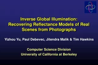
Inverse Global Illumination: Recovering Reflectance Models of Real Scenes from PhotographsYizhou Yu, Paul Debevec, Jitendra Malik, and Tim HawkinsSIGGRAPH ‘99 • 15-869, Image-Based Modeling and Rendering • Paul Heckbert, 20 Oct. 1999

Yu: Motivation • Most IBMR methods permit novel viewpoints but not novel lighting; they assume surfaces are diffuse. • Want to permit changes in lighting. • Would like to to recover (non-diffuse) reflectance maps: • specularity and roughness at each surface point

Yu: Simplifying Assumptions • static scene of opaque surfaces • known shape • known light source positions • calibrated cameras, known camera positions • high dynamic range photographs • specular reflection parameters (specular reflection coefficient and roughness) constant over large surface regions • each surface point captured in at least one image • each light source captured in at least one image • image of a highlight in each specular surface region in at least one photograph

Yu Algorithm Overview • 1. Solve for shape (use FAÇADE or similar system) • 2. Solve for coarse diffuse reflectances • coarsely mesh the surfaces into triangles • inverse radiosity problem: known form factors and radiosities (from image radiances), solve for diffuse reflectances (linear system) • 3. Solve for coarse specular reflectance • find highlights for each surface from known surface geometry & lights • check that highlight unoccluded • sample image at points around the highlight center • repeat until convergence • solve for diffuse and specular reflectances (linear system) for each region • solve for roughness of each region (nonlinear) • update estimates of interreflection between surfaces • 4. Solve for detailed diffuse reflectance (albedo maps) • look at all images of a given surface point, subtract specular component • throw out outlier (highlight-tainted values), average the rest

Yu: Acquisition Details • spherical, frosted light bulbs • 180 volt DC power to avoid 60Hz light flicker • black strips of tape on walls for digitization • shot 150 images with digital camera, merged to create 40 high dynamic range images (represent with floating point pixel values) • block light source to camera in some of the images • correct for radial distortion and vignetting

Light, Reflectance, and Global Illumination