1 / 0

Illumination and Light Transport

Cornell box rendered using photon mapping. Illumination and Light Transport. Chapters 29, 31, 33. Photo credit: Ben Herila , 2010. Outline. Photo source : http:// www.overclock.net/art-graphics/251218-kerkythea-shaded-lightsource-test.html. What is Light? Local vs. Global Illumination

apollo
Télécharger la présentation

Illumination and Light Transport

An Image/Link below is provided (as is) to download presentation Download Policy: Content on the Website is provided to you AS IS for your information and personal use and may not be sold / licensed / shared on other websites without getting consent from its author. Content is provided to you AS IS for your information and personal use only. Download presentation by click this link. While downloading, if for some reason you are not able to download a presentation, the publisher may have deleted the file from their server. During download, if you can't get a presentation, the file might be deleted by the publisher.

E N D

Presentation Transcript


  1. Cornell box rendered using photon mapping

    Illumination and Light Transport

    Chapters 29, 31, 33 Photo credit: Ben Herila, 2010
  2. Outline Photo source : http://www.overclock.net/art-graphics/251218-kerkythea-shaded-lightsource-test.html What is Light? Local vs. Global Illumination The Rendering Equation Illumination vs. Shading Computing Illumination Modeling Reflectance Illumination Models Shading Models Advanced Global Illumination Techniques October 31, 2013
  3. The Microscopic View of Light E2 E1 Light can be thought of as small packets of energy called photons Every atom has a nucleus which electrons orbit at various levels When an electron drops from a higher level orbit to a lower, energy (photons) are emitted (Planck’s Law) E=hf(frequency of emitted light increases with energy, h is Planck’s constant) When an emitted photon strikes another atom and is absorbed, electrons jump from a lower orbital to a higher one The wavelength (color) of light emitted or absorbed corresponds to the change in orbital. The nature of atoms and their electrons control the type of light emission See chapter 26 in book October 31, 2013
  4. The Microscopic View of Light Cloud Gate, Millenium Park, Chicago http://greghumphries.com/ Charcoal, source: http://budgetwarehouse.wordpress.com/party-needs/charcoal/ The different energy levels of electrons allow for different wavelengths of light to be reflected Metals have “loose” electrons which can move relatively freely and occupy many different energy levels, which is why they are more reflective Insulators have more constrained electrons which cannot change energy levels as easily, so they convert more absorbed light into heat instead of reflecting it October 31, 2013
  5. The Macroscopic View of Light Light is a type of electromagnetic radiation and can also be thought of as a continuous wave (as opposed to a discrete photon) The wave nature of light is best used to describe how light propagates or travels, whereas the particle description is best used to determine how energy is exchanged The wavelength of a wave is measured as the distance from the one peak of a wave to the next Visible light has a wavelength between about 400nm – 700nm, a very small portion of the entire spectrum Different wavelengths correspond to different colors; recall that all the cones in the retina react (non-uniformly) to all wavelengths in the visual spectrum October 31, 2013
  6. The Electromagnetic Spectrum Full electromagnetic spectrum Visible light has a wavelength between about 400nm – 700nm, tiny portion of spectrum We’re only interested in the visible spectrum – define and group major wavelength ranges, approximately red, green, and blue October 31, 2013
  7. Outline What is Light? Local vs. Global Illumination The Rendering Equation Illumination vs. Shading Computing Illumination Modeling Reflectance Illumination Models Shading Models Advanced Global Illumination Techniques October 31, 2013
  8. Illumination Models: Direct (non-global) Illumination Crudest hack: take only direct lighting information from light sources into account when computing a sample Usually involves an “ambient term” to set a sort of minimum bar for inter-object reflection and thus light up visible surfaces Used in OpenGL <3.0, most traditional hardware pipelines (“fixed function” as opposed to programmable shader- driven pipelines on modern GPUs) Nancy Tom’s Sceneview scene, rendered using OpenGL with only local illumination (2001). The fixed-function pipeline is deprecated in OpenGL 3.0, and removed in 3.1+ October 31, 2013
  9. Illumination Models: Global Illumination Simulates how other objects affect light reaching a surface element Lights and shadows most light striking a surface element comes directly from emissive light sources sometimes light from a source to a surface element is blocked by other objects; surface element is then in “shadow” from that light source classical h/w pipeline doesn’t account for blockers since each triangle is considered purely by itself Inter-object reflection (indirectillumination) light bounces off other objects toward our surface element, to add to direct illumination from Pixar’s “Luxo Jr.” October 31, 2013 indirect illumination object eye direct illumination light light object object
  10. Global Illumination + = Total illumination Direct illumination Indirect illumination October 31, 2013
  11. Diffuse Interreflection Total illumination (normal image) October 31, 2013
  12. Diffuse Interreflection Direct illumination October 31, 2013
  13. Diffuse Interreflection Indirect illumination (diffuse interreflection) October 31, 2013
  14. Human face Total illumination (normal image) October 31, 2013
  15. Human face Direct illumination October 31, 2013
  16. Human face Indirect illumination October 31, 2013
  17. How to separate direct and indirect components (1/3) Use a high frequency illumination pattern For example a checkerboard pattern of lit and unlit patches Each patch i that is not directly illuminated by the pattern should be lit due only to indirect illumination This gives an estimate for indirect illumination on patch i Algorithm Attribution: S. Nayar, G. Krishnan, M. Grossberg, and R. Raskar. “Fast Separation of Direct and Global Components of a Scene using High Frequency Illumination,” SIGGRAPH ‘06 October 31, 2013
  18. How to separate direct and indirect components (2/3) Then how do we estimate indirect illumination for patches that fall in a directly illuminated region? Light the scene by the complement of the original illumination pattern e.g., all lit squares in the checkerboard become unlit, and all unlit squares become lit Obtain estimate for direct illumination by subtracting the estimate for indirect illumination October 31, 2013
  19. How to separate direct and indirect components (3/3) In theory, a high frequency pattern and its complement are sufficient for separation. In practice, however, a series of images are used, each with the illumination pattern shifted slightly. This is because lit and unlit areas still have brightness variations due to inaccuracies in the projector. This technique can be applied to real life scenes use a projector to cast a shifting high frequency pattern and take multiple photographs is a technique from computer vision in that we are processing data captured from the real world Different illumination patterns can be used Checkerboard, sinusoidal pattern, line occluderpasses a narrow linear shadow across the scene Can produce impossible images which cannot be observed in the real world— adjust the blending ratio between indirect and direct illumination components October 31, 2013
  20. Video http://www.cs.columbia.edu/CAVE/projects/separation/videos/Separation.mov S. Nayar, G. Krishnan, M. Grossberg, and R. Raskar. “Fast Separation of Direct and Global Components of a Scene using High Frequency Illumination,” SIGGRAPH ‘06 October 31, 2013
  21. The Rendering Equation (Kajiya, Immel et al, 1986) Computing light transport in a scene with both direct light sources (emitters) and indirect sources, i.e., inter-object reflection – basically an energy balance: the radiance (energy) leaving a point is the sum of emitted and reflected light from other sources We compute integrals of the recursiveform is the radiance at surface point P in direction is the + hemisphere of all incoming directions to P. is one of those directions represents the amount of light emitted from the material at point P (zero for most objects) represents the BRDF term which is covered in more detail later in this lecture accounts for diminished intensity per unit area as a function of angle to the normal This equation is the foundation of almost all rendering algorithms (radiosity, photon mapping, path tracing…) It doesn’t handle subsurface scattering, phosphorescence and fluorescence; Also, the terms should include additional parameters for wavelength and time Image courtesy of: http://en.wikipedia.org/wiki/Rendering_equation October 31, 2013
  22. An Alternate Formulation of the Rendering Equation k S Light energy traveling from point i to j = light emitted from i to j (direct term), plus indirect term, light reflected from i to j. It is the integral over S of the value of the BRDF for every point k reflecting to i and from there to j times light energy L from k to i, all attenuated by a geometry factor G is the total amount of light (radiance)potentially traveling along the ray from point i to point j; occlusion not taken into account is the direct term, the amount of light emitted by the surface at point i (luminance) is the light reflected from i to j, this corresponds to the recursive integral of all indirect energy reflected from i is the Bidirectional Reflectance Distribution Function (BRDF) of surface at i. Describes fraction of light incident on surface at i from direction of k that leaves surface in direction of j – it is an attenuation factor between 0 and 1, and is a function of the reflection characteristics of the material. It can be measured for real materials is a geometry term which involves occlusion, distance, and angle between vectors; often 0 because of an occluder j i October 31, 2013
  23. Examples of Global Models The rendering equation takes into account global information of both direct (from emitters) and indirect illumination (inter-object reflections) Many different approximations with advantages and disadvantages, and their own resource requirements – in general, more computation gives better results Even purely local model is a zero’th order approximation to rendering eqn. Direct illumination + specular reflection Ray trace + soft shadows and caustics Ray trace + caustic photon map + diffuse reflection (color bleeding) Ray trace + caustic and diffuse photon maps http://graphics.ucsd.edu/~henrik/images/global.html October 31, 2013
  24. Illumination Models: Non-global vs. Global Models Direct (diffuse + specular) lighting + indirect specular reflection via recursiveray tracing Non-global models concentrate on light from direct sources pro: scene can be rendered fast con: pay a price in lost realism; lose interesting effects of light transport because we ignore effects of all other objects in the scene when considering a particular surface element Global models concentrate on capturing all illumination information pro: shadows, inter-object reflection, refraction, i.e. bending of light at translucent surfaces, caustics, volumetric effects of participating media such as air, water, fog, etc. con: slow Note that top image is darker because diffuse inter-object reflection is not counted, so no color bleeding. “Ambient” hack compensates for this difference Full global model using stochastic simulation for diffuse interreflections (color bleeding) Ray tracing + Light cache + Irradiance map October 31, 2013 http://www.spot3d.com/vray/help/200R1/examples_GI.htm
  25. Illumination Models: Non-global vs. Global Models Direct (diffuse + specular) lighting + indirect specular reflection Full global illumination October 31, 2013
  26. Illumination and Shading Lighting, or illumination, is the process of computing the intensity and color of a sample point in a scene as seen by a viewer lighting is a function of the geometry of the scene (including the model, lights and camera and their spatial relationships) and material properties Shadingis the process of interpolation of color at points in-between those with known lighting or illumination, typically vertices of triangles or quads in a mesh used in many real time graphics applications (e.g., games) since calculating illumination at a point is usually expensive. In ray-tracing only do lighting for samples (based on pixels or sub-pixel samples for super-sampling), no shading On the GPU processing triangles, lighting is calculated by a vertex shader, while shading is done by a fragment or pixel shader October 31, 2013
  27. Outline What is Light? Local vs. Global Illumination The Rendering Equation Illumination vs. Shading Computing Illumination Modeling Reflectance Illumination Models Shading Models Advanced Global Illumination Techniques October 31, 2013
  28. Illumination Models: Computing Illumination Illumination can be computed by: Light transport simulation: Evaluate illumination with enough samples to produce a final image without any guessing / shading, both for direct and for indirect components often used for high quality renderers, e.g., those used in FX movies some implementations can run in real time on the GPU, but more complex lighting models that are difficult to parallelize for GPUs are still run on the CPU renders of highest quality can take days for a single frame, even on modern distributed CPU render farms and/or GPU render farms Many simulations use stochastic sampling: path tracing, photon mapping, Metropolis light transport Polygon rendering: Evaluate illumination at several samples, and shade (using a shading model) in between to produce pixels in the final image often used in real-time applications such as computer games, done in GPU lower quality than light transport simulation, but can obtain satisfactory results with various additions such as maps (bump, displacement, environment), covered in upcoming lecture October 31, 2013
  29. Light Transport: Inverse Square Law In Ray assignment, account for light attenuation (affects all models) Amount of light that illuminates an object decreases with square of distance between them For a given 3D angle (solid angle), the area it covers grows with the square of the distance Intensity of light per unit area falls off with the inverse square Conversely, for a fixed area, the angle it covers decreases with the square of the distance Slide 45 shows a hack that produces better results October 31, 2013
  30. Outline bubble with reflection, by d ha rm e sh What is Light? Local vs. Global Illumination The Rendering Equation Illumination vs. Shading Computing Illumination Modeling Reflectance Illumination Models Shading Models Advanced Global Illumination Techniques October 31, 2013
  31. Modeling Reflectance: The BRDF (1/2) Light arriving at a surface can scatter in many directions The direction of scattering is determined by the material Intensity at a given outgoing direction is dependent on incoming direction and material properties (how much energy it absorbs, how much it reflects diffusely vs. specularly, etc.) Model or measurement of reflectance is called thebidirectional reflectance distribution function (BRDF): for any incoming light ray how much energy is reflected for any outgoing light ray + = BRDF for simple model of diffuse + specular reflection, e.g., the Phong Lighting Model Total Scattering Distribution (BRDF) Specular Reflections Diffuse Reflections October 31, 2013
  32. Modeling Reflectance: The BRDF (2/2) When light hits a surface, it can be reflected, refracted, absorbed, or otherwise scattered (e.g., subsurface scattering) BRDF represents material properties of an object and how it reflects light Given an incoming direction, outgoing direction, incident point on object, and properties of lights, BRDF provides how much light reflects off surface can be measured with equipment or estimated based on some model Note that the BRDF is often implicit in simplest illumination models, and a few parameters (typically diffuse and specular reflection coefficients) are adjusted experimentally until desired visual outcome is achieved For this course, primarily concern ourselves with simple reflectance models October 31, 2013
  33. Simple Reflectance Models Some of these models you have seen before in OpenGL Lambertian light scatters equally (output radiance is equal) in all outgoing directions (i.e. viewer independent) Diffuse light scatters (possibly unevenly) in all outgoing directions, e.g., rug, paper, unvarnished wood Mirrorlight scatters in a single direction, Specular light scatters tightly around a particular direction (shiny objects with sharp highlights) Glossy light scatters weakly around a particular direction ωr n ω October 31, 2013
  34. Modeling Reflectance: Lambertian (1/2) As angle between light and normal increases , light’s energy spreads across a larger area is intensity (light’s color) of directional light (rays parallel to l) 3D visualization: hemisphere represents equal magnitude of reflected intensity for any outgoing vector. Real surfaces will have asymmetric BRDFs. Lambertian surfaces have uniform, diffuse-only scattering;same apparent brightness independent of view direction and incoming light direction Most materials are not perfectly Lambertian; most BRDFs are viewer dependent Lambert’s cosine law: l) October 31, 2013
  35. Modeling Reflectance: Lambertian (2/2) Several lighting models attempt to approximate these phenomena Models you have seen before– no physical foundation, but looks okay Phong Model Blinn-Phong Model Some more complicated models are physically based Cook-Torrance Model Oren-Nayer Model Which model we use largely depends on our application Usually a performance vs. accuracy tradeoff October 31, 2013
  36. Modeling Reflectance: Specular Most materials are not perfectly Lambertian; most BRDFs are viewer dependent this is the specularproperty of the material BRDF value is greatest when (when the outgoing angle is opposite the incoming angle ), like a perfect mirror or rippling water October 31, 2013
  37. Modeling Reflection: BSSRDF Image: No scattering (top) vs. with BSSRDF scattering (bottom). Image credit: http://graphics.ucsd.edu/~henrik/images/subsurf.html All of these models model light when it hits a surface directly and then scatters Light may also be scattered/absorbed while traveling through participating media (e.g., fog) The BRDF can be generalized to model transmission through an object (i.e. refraction) and sub-surface scattering by defining other terms, such as the bidirectional scattering surface reflectance distribution function (BSSRDF) October 31, 2013
  38. Modeling Reflectance: Subsurface Scattering Some surfaces may also reflect light internally a little before letting the light escape again (subsurface scattering) marble, skin, wax, hair, milk and other fluids More complex models are needed to approximate these interactions October 31, 2013
  39. Modeling Reflectance: Measuring B*DFs Image credit: Chuck Moidel Researchers collect tables of data for B*DFs of specific materials using devices like the one pictured The basic idea is to vary a light source around a hemisphere and measure the intensity at that direction. October 31, 2013
  40. Outline What is Light? Local vs. Global Illumination The Rendering Equation Illumination vs. Shading Computing Illumination Modeling Reflectance Illumination Models Shading Models Advanced Global Illumination Techniques October 31, 2013
  41. Illumination Models: Phong (1/5) (Review) Simple model (not physically based) Splits illumination at a surface into three components Ambient – Non-specific constant global lighting (hack) Diffuse – Color of object under normal conditions using Lambert’s model Specular – Highlights on shiny objects (hack) Proportional to so a larger results in a more concentrated highlight and glossier object October 31, 2013
  42. Illumination Models: Phong (2/5) (Review) Variables λ = color component (approximated by just using three eqn’s for R, G, and B) i = intensity of light as measured at surface ia= the amount of ambient light used in the scene k = material's efficiency at reflecting light (attenuation coefficient) ka is the ambient attenuation coefficient for this object's material kd is the diffuse attenuation coefficient for this object’s material (expect ka≃ kd) O = innate color of object's material at specific point on surface October 31, 2013
  43. Illumination Models: Phong (3/5) (Review) Ambient component effect on surface constant regardless of orientation, no geometric information total hack (crudest possible approximation to inter-object reflection), but makes all objects a little visible Diffuse component uses Lambert's diffuse-reflection cosine law (light's intensity) and ℓ (light's direction) vary for each light source kaandkdare ambient and diffuse attenuation coefficients – typically the same = innate color of object's diffuse material property at specific point on surface = innate color of the object’s ambient material property at specific point on surface, typically same as Both k and O are non-physical, dimensionless fractions between 0 and 1 October 31, 2013
  44. Illumination Models: Phong (4/5) (Review) The full Phong model is a combination of ambient, Lambertian and specular terms (summing over all the lights) Subscript represents specular (so ) is specular coefficient is the reflected direction of the light ray about the surface normal the smaller the angle δbetween V and R, the brighter reflection is the lighting attenuation function function of distance from the light Note: for a directional light, lis simply a directional vector. For a point light,lmust be computed from the light’s positions and the surface point. October 31, 2013
  45. Illumination Models: Phong(5/5) (Review) By the inverse square law, density of light energy decreases by the inverse square of the distance from the surface, due to spherical radiation pattern, so , where This will attenuate the light intensity according to distance, so farther objects appear darker, i.e. surfaces with equal vary in appearance if they are at different distances from the light – important if two surfaces overlap But this doesn’t look good – objects illuminated by point lights will look as if they were very harshly lit (things get dark too fast) Instead, use the following heuristic (hack) where c1, c2, c3 are experimentally-defined constants October 31, 2013
  46. Illumination Models: Blinn-Phong Variation on Phong model which modifies the specular term to be more computationally efficient The new specular term uses the half angle between the viewer and the light (not a function of the orientation/normal) instead of the angle between the reflected light ray and the viewer is the half angle l is normalized direction from point to light, V is normalized vector to viewer Use Blinn-Phong or Phong? Doesn’t matter, they look slightly different but they’re both hacks - October 31, 2013
  47. Illumination Models: Computing Results Look closely at the specular term: We can compute this term recursively shoot a ray from eye through a pixel on the screen calculate intersections of ray with all primitives in the scene, pick the closest one shoot a specular reflection ray from the intersection point to closest object to calculate its specular contribution. Spawn a secondary specular ray, etc. apply our simple illumination model at every intersection point, accounting for direct contribution from non-occluded lights, and indirect specular contributions from nearest objects can even be done in hardware thanks to modern GPU’s This is recursive Ray Tracing – simple global model that only computes specular inter-object reflection You will be implementing this soon October 31, 2013
  48. Outline What is Light? Local vs. Global Illumination The Rendering Equation Illumination vs. Shading Computing Illumination Modeling Reflectance Illumination Models Shading Models Advanced Global Illumination Techniques October 31, 2013
  49. Shading Models – Flat/Constant (Review) We define a normal at each polygon (not at each vertex) Lighting: Evaluate the lighting equation at the center of each polygon using the associated normal Shading: Each sample point on the polygon is given the interpolated lighting value at the vertices (i.e. a total hack) October 31, 2013
  50. Shading Models – Gouraud (Review) An issue with Gouraud shading is that specular highlights appear to “jump” as the object rotates. Simple fix is to increase polygon count, at cost of much more computation. Define a normal vector at each vertex Lighting: Evaluate lighting equation at each vertex using associated normal vector Shading: Each sample point’s color on polygon is interpolated from color values at polygon’s vertices October 31, 2013
  51. Shading Models – Phong (Review) Each vertex has an associated normal vector Lighting: Evaluate lighting equation at each vertex using associated normal vector Shading: For every sample point on polygon we interpolate normalsat vertices of the polygon and compute color using lighting equation with the interpolated normal at each interior pixel – more accurate representation of true surface normal at each point (and we don’t get moving specular highlights) October 31, 2013
  52. Outline What is Light? The Rendering Equation Illumination vs. Shading Local vs. Global Illumination Computing Illumination Modeling Reflectance Illumination Models Shading Models Advanced Global Illumination Techniques October 31, 2013
  53. Advanced GI Techniques In practice, calculating global illumination for a scene is a very complex and computationally intensive task Many algorithms (both real time and non real time) have been developed to calculate or approximate global illumination Real time Ambient occlusion, image based lighting Not (yet) real time Radiosity (intro later), Metropolis light transport, photon mapping, point based color bleeding October 31, 2013
  54. Advanced GI Techniques Advanced GI Techniques Photon Mapping Mental Ray RendererBioshock 2 Determine amount of light at a point by sending packets of energy (photons) from each light source out into the scene and counting how many are around that point. Photon Mapping Mental Ray RendererBioshock 2 Determine amount of light at a point by sending packets of energy (photons) from each light source out into the scene and counting how many are in neighborhood around that point.
  55. Advanced GI Techniques Advanced GI Techniques Point-Based Color Bleeding Renderman RendererUp! First generates a direct illumination point cloud. Uses the point cloud for lookup during rendering to approximate diffuse light bounces by adding up the contribution from other points in the cloud. Point-Based Color Bleeding Renderman RendererUp! First generates a direct illumination point cloud. Uses the point cloud for lookup during rendering to approximate diffuse light bounces by adding up the contribution from other points in the cloud.
  56. Advanced GI Techniques Advanced GI Techniques Image Based Lighting Sunflow RendererShiny Aliens Take a picture of a mirrored sphere in some environment, and use the color on the sphere to determine the global illumination in the scene Image Based Lighting Sunflow RendererShiny Aliens Plot an image onto a dome or sphere, using the lighting properties of this surface to determine global illumination when rendering the scene.
More Related