Illumination
Illumination. Behaviour of light. Shading Overview. Classical real-time shading: vertices projected to screen lighting calculation done at each vertex results interpolated along line (linear interpolation) to interior of polygon (bilinear interpolation) per-pixel shading:

Illumination
E N D
Presentation Transcript
Illumination Behaviour of light
Shading Overview Classical real-time shading: vertices projected to screen lighting calculation done at each vertex results interpolated along line (linear interpolation) to interior of polygon (bilinear interpolation) per-pixel shading: uses interpolated values and texture lookups as input into program that calculates pixel color
Classic Lighting Model Actual behavior of light extremely complex Widely used simplification in graphics: diffuse lighting matte surface directional light specular lighting shiny surface directional light ambient lighting omnidirectional light
Three-term Lighting Model Shading calculation done with three components: diffuse (Lambertian) direct lighting Id = N • L specular direct lighting Is = (V • R)^n ambient Ia = c
Diffuse component Matte objects: “not at all shiny” chalk, paper, rough wood, concrete Intensity of reflected light depends on angle between light source and surface normal Does not depend on viewing direction
Diffuse component Id = N • L N is surface normal L is direction towards light N L
Specular component Highlights on “shiny” (highly reflective) surfaces Intensity depends on angle between viewing direction and direction of ideal reflection
Specular component Given viewing direction and reflection direction, find cosine of angle between (by taking dot product) and raise to a power Lower powers give more spread-out highlights, and higher powers focus the highlight Is = (V • R)^n
Specular Component Is = (V • R)^n V is view direction R is reflection direction V R
Highlight spread dot product of normalized vectors is cosine of angle between vectors (V • R)^n = (cos α)^n Parameter n controls width of highlight: low n (say 1-5): broad highlight large n: (say 30-200): sharp highlight
Specular component How to compute reflection direction? R = -L + 2*(L • N)N
Ambient component Some amount of light always present Add small constant light intensity Just a hack to account for scattered light reaching everywhere Ambient occlusion: small-scale self-shadowing, can be precomputed (static scene) or computed in real time (SSAO, Crysis)
Three-term Lighting Model Shading calculation done with three components: I = kd(N • L) + ks(V • R)^n + ka k is surface albedo Actually have three such equations, one each for R, G, and B Not shown: lighting modulated by color of surface (material properties), incoming light
3-term lighting "Phong" because per-pixel lighting
Light Attenuation Light intensity falls off with distance from source 1/r^2 physically correct for point sources, but works poorly in practice hacked 1/(c1 + c2r + c3r^2) sometimes used Atmospheric haze: cue for large distances
Interpolation Remember – information available only at vertices Classically, lighting calculation done only at vertices also Need to interpolate to remainder of primitive flat shading also possible
Linear Interpolation Linear interpolation: simplest method to interpolate i(t) = i(0)*(1-t) + i(1)*t, t in (0,1) values known at 0 and 1, interpolated otherwise Widely used – here just for shading lines
Gouraud Shading Compute illumination at vertices Bilinearly interpolate to interior Gouraud shading proper: compute surface normals from polygon (cross product) average all polygon normals touching vertex to obtain vertex normal
Phong Shading Lighting can change faster than geometry With insufficient vertex density, features can be missed Phong shading: interpolate normals to triangle interior perform per-pixel lighting Much more costly but better effect
Phong vs Gouraud shading Historically, Gouraud usually used in real-time graphics "why do all video games look the same?" Now, pixel shaders are the norm – per-pixel lighting possible (expected)
Custom Shading With the advent of programmable shaders, we are no longer restricted to the 3-term lighting model Pixel shaders now standard Phong shading other, specialized lighting models, effects
What is color, anyway? • We think of it as a property of an object • “blue shirt”, etc. • Complex relationship between properties of material, lighting conditions, and properties of receptor • in graphics, need to account for properties of display device as well (monitor, printer)
Human Color Vision • Cones: three types – red (rho), green (gamma), blue (beta) • Rho: 64% of cones • Gamma: 32% of cones • Beta: only 2% of cones, present outside foveal region • Rho and Gamma spectral sensitivities overlap considerably
Metamerism • Possible for distinct spectra to evoke the same sensor response • Metamers: sets of spectra which are perceived as the same color • Human vision system has 3 receptor types, so three-dimensional color space needed
3D color space • RGB: most common in graphics, tied to output capabilities of CRT monitors
RGB • Additive color model • light • Primary colors: R, G, B • (x,0,0), (0,x,0), (0,0,x) • Secondary colors: yellow, magenta, cyan • (x,x,0), (x,0,x), (0,x,x) • Host of other colors
CMYK • Cyan, Magenta, Yellow, blacK (key) • subtractive color model for ink
Three-term Lighting Model I = kd(N • L) + ks(V • R)^n + ka Important quantities: material of surface normal vector shininess light direction, eye direction Where they come from property of model/configuration interpolated from vertex stored in texture (or computed procedurally)
Toon Shading • Shading style characterized by • large flat-colored regions • "shading" quantized into few colors • black outlines denoting • silhouettes • internal object boundaries • (eg, eyes) • creases • Recent toonshaders often omit outlines
Quantized Shading • Create 1D texture map showing progression of colors • Calculate lighting as normal (diffuse+specular) • Use lighting result to index into texture • If only few colors, can use if statements • bad for reusability, good for rapid prototyping
Outlines • Silhouettes: where depth differences exceed a threshold • can render to texture and find depth differences in second pass of pixel shader • Boundaries: property of model, annotated • Creases: property of model • could be annotated (artist, precomputed) • could be obtained by differencing normal map in pixel shader
Local Illumination • Considers only information at shaded point on surface • Traditionally, 3-term lighting model • Missing many elements that contribute to appearance of surface • indirect lighting • shadows • subsurface scattering, participating medium
Subsurface Scattering [Wann Jensen, 2001]