NCL for WRF Model Output
NCL for WRF Model Output. The NCL scripts for plotting WRF model output are our first cut at producing plots for use in our development efforts. The scripts do not constitute and analysis package. NCL is an interpreted language allowing for fast and easy

NCL for WRF Model Output
E N D
Presentation Transcript
NCL for WRF Model Output The NCL scripts for plotting WRF model output are our first cut at producing plots for use in our development efforts. The scripts do not constitute and analysis package. NCL is an interpreted language allowing for fast and easy prototyping, built in capabilities to easily read and write a variety of data formats, complete NCAR Graphics capabilities, and easy linking to Fortran and C routines. Thus we may build an analysis package based on NCL in the future. Don’t be shy about digging into the scripts!
Using NCL with WRF Model Output Step 1: After downloading WRF-NCL tar file (wrf_plot_ncl.tar), build the fortran shared library using the script “make_ncl_fortran”. Step 2: Place the WRF output file into the ncl directory with the scripts. Step 3: Edit one of the scripts for producing the desired WRF plots, setting the appropriate input file name And desired output format. Step 4: Run the script: “ncl < script”
Example WRF NCL Plotting Script ; ; script to produce standard plots for a wrf real-data run ; load "wrf_plot.ncl" load "wrf_user.ncl" load "gsn_code.ncl" load "skewt_func.ncl" a = addfile("wrfout_01_000000.nc","r") ;wks = wrf_open_X11() ; output to screen wks = wrf_open_ncgm("wrf_plots") ; output to ncgm ;wks = wrf_open_PS("wrf_plots") ; output to postscript frame(wks) ; allow for window resize before beginning plots times = wrf_user_list_times(a) ; get times in the file pressure_levels = (/ 850., 700., 500., 300./) ; pressure levels to plot ntimes = dimsizes(times) ; number of times in the file nlevels = dimsizes(pressure_levels) ; number of pressure levels Files containing NCL functions and routines open netcdf file output options
Example WRF NCL Plotting Script (cont.) Loop through all times in the output file do it = 0, ntimes-1 time = it print(times(it)) if (it.eq.0) then time_save = times(it) end if hours = it*6. ; start with surface pressure plot slvl = wrf_user_getvar(a,"slvl",time) ; psl wrf_user_filter2d(slvl, 3) ; filter the fields tc = wrf_user_getvar(a,"tc",time) tc = 1.8*tc+32. u = wrf_user_getvar(a,"ua",time) ; ua is u averaged to mass points v = wrf_user_getvar(a,"va",time) ; va is v averaged to mass points u = u*1.94386 v = v*1.94386 tc_plane = tc(0,:,:) u_plane = u(0,:,:) v_plane = v(0,:,:) Function (wrf_user_getvar) that reads data from the WRF output file and computes appropriate diagnostic fields (if necessary)
Example WRF NCL Plotting Script (cont.) opts_tc = True opts_tc@MainTitle = "Surface T (F, color) SLP (mb) and winds (kts)" ; and many more options... opts_psl = True ; and many more options... opts_vct = True opts_vct@NumVectors = 47 opts_vct@WindBarbsOn = True opts_vct@NoTitles = True opts_vct@vcWindBarbColor = "black" opts_vct@vcRefAnnoOn = False opts_mp = True ; and many more options... map = wrf_new_map(wks,a,opts_mp) opts_map = True opts_map@LabelFont = "HELVETICA-BOLD" opts_map@LabelFontHeight = .01 wrf_maplabel(wks,map,opts_map) Options for plots. Logical variable is “True” if options are present, options are attributes of the logical variable Create map background, label map
Example WRF NCL Plotting Script (cont.) Create plots (contour fill/line and vector) contour_tc = wrf_new_fill_contour(wks,tc_plane,opts_tc) contour_psl = wrf_new_line_contour(wks,slvl(:,:),opts_psl) vector = wrf_new_vector(wks,u_plane, v_plane,opts_vct) wrf_mapoverlay(map,contour_tc) wrf_mapoverlay(map,contour_psl) wrf_mapoverlay(map,vector) draw(map) frame(wks) Combine individual plots into single picture (overlay or merge) Send picture to output device Clear for the next picture
Example WRF NCL Plotting Script (cont.) ; preparing for 3-D plots p = wrf_user_getvar(a, "p",time) ; pressure is our vertical coordinate z = wrf_user_getvar(a, "Z",time) ; grid point height rh = wrf_user_getvar(a,"rh",time) w = wrf_user_getvar(a,"wa",time) w = 100.*w tc = (tc-32.)*.55555 do level = 0,nlevels-1 pressure = pressure_levels(level) z_plane = wrf_user_intrp3d( z,p,ter,"h",pressure,0.) tc_plane = wrf_user_intrp3d(tc,p,ter,"h",pressure,0.) u_plane = wrf_user_intrp3d( u,p,ter,"h",pressure,0.) v_plane = wrf_user_intrp3d( v,p,ter,"h",pressure,0.) rh_plane = wrf_user_intrp3d( rh,p,ter,"h",pressure,0.) w_plane = wrf_user_intrp3d( w,p,ter,"h",pressure,0.) ; lots of plotting... end do Loop over desired pressure surface for plots Vertical interp to desired surface
Example WRF NCL Plotting Script (cont.) Vertical cross sections do ip = 1, 2 dimsrh = dimsizes(rh) plane = new(2,float) plane = (/ dimsrh(2)/2, dimsrh(1)/2 /) if(ip .eq. 1) angle = 90. else angle = 0. end if rh_plane = wrf_user_intrp3d(rh,z,ter,"v",plane,angle) tc_plane = wrf_user_intrp3d(tc,z,ter,"v",plane,angle) ; lots of plotting... end do Point in model ‘gridpoint’ space Angle of plane passing through ‘gridpoint’ Interpolation to vertical cross section
Example WRF NCL Plotting Script (cont.) qv = wrf_user_getvar(a,"QVAPOR",time) td = wrf_user_getvar(a,"td",time) u = wrf_user_getvar(a,"umet",time) v = wrf_user_getvar(a,"vmet",time) u = u*1.94386 v = v*1.94386 ; bunch of options locr = wrf_user_find_ij_lat_long(a, 39.77, 104.87 ) loc = floattointeger(locr) loc_str = "Skew-T at Denver valid at " + times(it) skewt_bkgd = skewT_BackGround (wks, skewtOpts) draw (skewt_bkgd) skewT_data = skewT_PlotData(wks, skewt_bkgd, p(:,loc(0), loc(1)), \ tc(:,loc(0), loc(1)), \ td(:,loc(0), loc(1)), \ z(:,loc(0), loc(1)), \ -u(:,loc(0), loc(1)), \ -v(:,loc(0), loc(1)), \ dataOpts ) frame(wks) end do end do Skew-T plots First get necessary variables Find nearest gridpoint Options needed (skewOpts) not shown here
NCL for WRF Model Output The NCL scripts for plotting WRF model output are our first cut at producing plots for use in our development efforts. The scripts do not constitute and analysis package. NCL is an interpreted language allowing for fast and easy prototyping, built in capabilities to easily read and write a variety of data formats, complete NCAR Graphics capabilities, and easy linking to Fortran and C routines. Thus we may build an analysis package based on NCL in the future. Don’t be shy about digging into the scripts!