WRF model exercise
WRF model exercise. Experimental Boundary layer meteorology Björn Claremar 2012. Outline. Why use models ? The WRF model Physics schemes The computer lab. Use of models. Observations are not always sufficient to find out meteorology between observational stations.

WRF model exercise
E N D
Presentation Transcript
WRF model exercise Experimental Boundary layer meteorology BjörnClaremar 2012
Outline • Whyusemodels? • The WRF model • Physicsschemes • The computer lab
Use of models • Observations are not always sufficient to find out meteorology between observational stations. • Meteorological re-analysis data are good to fill in gaps between observations (e.g. NCEP, ERA-40, ERA-Interim) • Numerical weather model makes sub-sequent short-range forecast with observations (at ground and in free atmosphere) as initial and boundary forcing • too coarse resolution (>80 km) to catch the influences on weather from the complex topography.
Regional modelling gives more detail Simulated precipitation GCM 300 km GCM interp. to 50 km RCM 50 km
RCA3 with higher resolution Precipitation (DJF, 1987-2007) as a function of resolution
Downscaling processERA-Interim re-analysis • Gridded dataset, partly based on: • Direct meteorological observations and satellite measurements • Prognostic atmospheric model • Assimilation of observations to physical consistent fields. • Precipitation fully prognostic • Data available from 1990 and onwards.
Downscaling processWRF3 model • Developed at National Center for Atmospheric Research (NCAR) • Equations: Fully compressible, Euler non-hydrostatic, conservative for scalar variables. • Vertical Coordinate: Terrain-following. • Physics schemes: interchangeable • This study • Running WRF3 with ERA-Interim at the boundaries (3-D fields and near surface parameters) and below (SST/ice/snow) to 8 and 2.7 km grid and 27 vertical levels. 2.7 km WRF Terrestrial data 30’’ Preprocessing and initialization Advanced Research WRF ERA-Interim (6 h) 200 m contour lines
Preliminary results (standard WRF)- precipitation • Precipitation becomes more influenced by the terrain and increases more than 100% locally. • Precipitation is much larger in WRF compared to ERA-Interim (too much? Better with polar physics?) ERA-Interim WRF Mean yearly precipitation 2000-2008 (mm)
Results – wind case WRF ERA-Interim 1100 m (m/s) • Geostrophic wind (not influenced by surface friction) • Finer details • 10-m • Finer details • Increase of wind at mountain tops and as channeling and corner effects (note southern tip) • Decrease of wind in lee areas Geostrophic (m/s) 10 m (m/s) 10 m (m/s)
Nordaustlandet • 10 m-wind • Lee in valleys and maxima over the ice sheet • Distinct katabatic winds and channeling
What is WRF • http://wrf-model.org/index.php • The Weather Research and Forecasting (WRF) is developed at National Center for Atmospheric Research (NCAR) • Designed to serve both operational forecasting (NMM) and atmospheric research needs (ARW). • Physics and dynamics schemes are interchangeable • Features multiple dynamical cores, a 3-dimensional variational (3DVAR) data assimilation system, and a software architecture allowing for computational parallelism and system extensibility. (Not used here) • WRF is currently in operational use at NCEP, AFWA and other centers
Dynamical equations • fully compressible • Non-hydrostatic (with a runtime hydrostatic option). • vertical coordinate is a terrain-following hydrostatic pressure coordinate. grid-spacing can vary with height • Grid staggering is the Arakawa C-grid. • u components at the centers of the left and right grid faces, and the v components at the centers of the upper and lower grid faces • Runge-Kutta 2nd and 3rd order time integration schemes, and 2nd to 6th order advection schemes in both horizontal and vertical. • time-split small step for acoustic and gravity-wave modes. The dynamics conserves scalar variables. • 1- or 2-way nesting available • Moving nests (prescribed moves and vortex tracking) • nudging
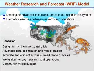
Application fields • suitable for a broad spectrum of applications across scales ranging from meters to thousands of kilometers. Idealized simulations (e.g. LES, convection, baroclinic waves) • Parameterization research • Data assimilation research • Forecast research • Real-time NWP • Hurricane research • Regional climate research (dynamical downscaling) • of re-analysis fields or atmosphere-ocean coupled general circulation models (AOGCMs) • Coupled-model applications • Teaching
7 different physics types Descriptions and references at http://www.mmm.ucar.edu/wrf/users/docs/user_guide_V3/users_guide_chap5.htm#Phys • Long wave radiation physics • Short wave radiation physics • Cumulus physics (small scale convective clouds) (important only over sea in the Arctic) • Land-surface model We concentrate on: • Cloud physics (microphysics): simulates cloud and precipitation processes • Boundary layer physics • Surface layer physics
Present land surface model (LSM) in WRF 4 soil layers (10, 30, 60, 100 cm) Soil layers can turn into snow layers Runoff and infiltration
Polar WRF • The key modifications for Polar WRF are in the land surfacemodel (LSM) Noah : • Optimal surfaceenergybalanceand heat transfer over seaice and permanent icesurfaces • Implementation of a variable seaicethickness and snowthickness over seaice • Implementation of seasonally-varingseaicealbedo • Alsospecificphysicssuitable for Arctic conditions (in dark blur in followingslides)
Microphysics (mp_physics) • X-class: number of different “particles” • Single-moment: Particlemixingratio • Double-moment: Particlemixingratio + particelnumberconcentration Some examples Single moment • c. WRF Single-Moment 3-class scheme: A simple, efficient scheme with ice and snow processes suitable for mesoscale grid sizes (3). • d. WRF Single-Moment 5-class scheme: A slightly more sophisticated version of (c) that allows for mixed-phase processes and super-cooled water (4). • e. Eta microphysics: The operational microphysics in NCEP models. A simple efficient scheme with diagnostic mixed-phase processes. For fine resolutions (< 5km) use option (5) and for coarse resolutions use option (95). • f. WRF Single-Moment 6-class scheme: A scheme with ice, snow and graupel processes suitable for high-resolution simulations (6). Double-moment • h. New Thompson et al. scheme: A new scheme with ice, snow and graupel processes suitable for high-resolution simulations (8). This adds rain number concentration and updates the scheme from the one in Version 3.0. New in Version 3.1. • j. Morrison double-moment scheme (10). Double-moment ice, snow, rain and graupel for cloud-resolving simulations. New in Version 3.0. • k. WRF Double-Moment 5-class scheme (14). This scheme has double-moment rain. Cloud and CCN for warm processes, but is otherwise like WSM5. New in Version 3.1. • l. WRF Double-Moment 6-class scheme (16). This scheme has double-moment rain. Cloud and CCN for warm processes, but is otherwise like WSM6. New in Version 3.1.
Surface Layer (sf_sfclay_physics) Scheme must be working with PBL physics • a. MM5 similarity: Based on Monin-Obukhov • with Carslon-Bolandviscoussub-layer • standard similarityfunctions from look-uptables (sf_sfclay_physics = 1). • b. Etasimilarity: Used in Etamodel. Based on Monin-Obukhov • with Zilitinkevichthermalroughnesslength • standard similarityfunctions from look-uptables (2). • d. QNSE surfacelayer. Quasi-NormalScale Elimination PBL scheme’ssurfacelayer option (4). • new theory for stably stratified regions • e. MYNN surfacelayer. Nakanishi and NiinoPBL’ssurfacelayerscheme (5). • Includesbetter interaction of the turbulence with microphysics and radiation in the PBL, compared to the MYJ2.5 scheme
PBL turbulenceclosure • First order closure (K-theory): 2nd order moments are parameterized • 1.5 order closure • TKE and potential temperature variance budgets • KM = f(TKE,q’ variance) • Higher order closures • Only higher order moments are parameterized • Example: 2nd order closure uses budgets for 2nd order moments and parameterizes 3rd order moments, dissipation terms and pressure gradient correlations
4. PlanetaryBoundarylayer (bl_pbl_physics) • a. Yonsei University scheme: Non-local-Kscheme with explicit entrainmentlayer and parabolic K profile in unstable mixed layer (bl_pbl_physics = 1). • b. Mellor-Yamada-Janjicscheme (MYJ2.5): Etaoperationalscheme. One-dimensionalprognostic turbulent kineticenergyscheme with localverticalmixing (2). • e. Quasi-NormalScale Elimination PBL (4). A TKE-prediction option that uses a new theory for stablystratifiedregions. Daytime part useseddydiffusivitymass-fluxmethod with shallowconvection (mfshconv = 1) which is added in Version 3.4. • f. Mellor-YamadaNakanishi and Niino (MYNN) Level 2.5 PBL (5). • Predictssub-grid TKE terms. • Includesbetter interaction of the turbulence with microphysics and radiation in the PBL, compared to theMYJ2.5 scheme
QNSE scheme for PBL/surfacelayer(Quasi-NormalScaleElimination) • k-e model • uses a new theory for stably stratified regions. accounts for anisotropic turbulence and gravity waves and is not based on the shortcomings of Reynolds stress models in verystablestratifications.
Computer lab • Run WRF model during 36 h with different physical parameterizations and vertical resolution. • You are also welcome to extend the test if you have time!
Look at: • time evolution of temperature at Nordenskiöldbreen in comparison to measurements. • time evolution of wind speed at Nordenskiöldbreen in comparison to measurements. • time evolution of temperature profile • time evolution of wind profile
Running WRF • You will use the KALKYL computer cluster at UPPMAX • The environment is scientific Linux and you will reach the system via the program Putty and WinSCP • In Putty you can run the programs • WinSCP is better to use when downloading data and changing in text files. • You will do your analyses in MATLAB (or excel).
UPPMAX • Uppsala Multidisciplinary Center for Advanced Computational Science (UPPMAX) is Uppsala University's resource of high-performance computers, large-scale storage, and know-how of high-performance computing (HPC). The center is a member of the national metacenter Swedish National Infrastructure for Computing (SNIC). • UPPMAX was founded in 2003, but builds on a much longer successful history of HPC activities at Uppsala University. • UPPMAX is hosted by the Department of Information Technology, Faculty of Science and Technology at Uppsala University and is one of the six centra in the national metacenter Swedish National Infrastructure for Computing (SNIC). • UPPMAX is part of the SweGrid national grid. • UPPMAX is funded by the Faculty and by SNIC.
The KALKYL cluster • TechnicalSummary • 348 ComputeNodes with 2784 CPU cores • 9504 Gigabyte total RAM • 113 Terabyte total disk • interconnected with a 4:1 oversubscribed DDR Infinibandfabric • 696 CPU's in 348 dual CPU, quadcore, nodes • HP SL170h G6 compute servers • Quad-core Intel® Xeon 5520 (Nehalem 2.26 GHz, 8MB cache) processors • 316 nodes with 24 GB memory and 250 GB hard disk • 16 nodes with 48 GB memory and 250 GB hard disk • 16 nodes with 72 GB memory and 2 TB hard disk
Downscaling processWRF3 model • This study • Running WRF with ERA-Interim at the boundaries (3-D fields and near surface parameters) and below (SST/ice/snow) to 24 and 8 km grid and 27 vertical levels. 2.7 km WRF Terrestrial data 30’’ Done! Preprocessing and initialization Advanced Research WRF ERA-Interim (6 h) 200 m contour lines
Namelist • &time_control • run_days = 0, • run_hours = 1, • run_minutes = 0, • run_seconds = 0, • start_year = 0001, • start_month = 01, • start_day = 01, • start_hour = 00, • start_minute = 00, • start_second = 00, • end_year = 0001, • end_month = 01, • end_day = 01, • end_hour = 01, • end_minute = 00, • end_second = 00, • history_interval = 10,
Namelist • &domains • time_step = 3, • time_step_fract_num = 0, • time_step_fract_den = 1, • max_dom = 1, • s_we = 1, • e_we = 202, • s_sn = 1, • e_sn = 3, • s_vert = 1, • e_vert = 81, • dx = 250, • dy = 250, • p_top_requested= 5000, • eta_levels= 1.000, 0.997, 0.993, 0.988, 0.982, • 0.975, 0.965, 0.952, 0.937, 0.917, • 0.891, 0.860, 0.817, 0.766, 0.707, • 0.644, 0.576, 0.507, 0.444, 0.380, • 0.324, 0.273, 0.228, 0.188, 0.152, • 0.121, 0.093, 0.069, 0.048, 0.029, • 0.014, 0.000,
Namelist • &physics • mp_physics = 2, • ra_lw_physics = 0, • ra_sw_physics = 0, • radt = 0, • sf_sfclay_physics = 0, • sf_surface_physics = 0, • bl_pbl_physics = 0, • bldt = 0, • cu_physics = 0, • cudt = 0, • isfflx = 0, • ifsnow = 0, • icloud = 0, • num_soil_layers = 5, • mp_zero_out = 0,