Greedy Algorithms
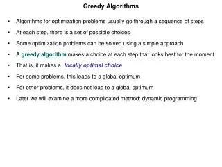
Greedy Algorithms. Greedy Algorithms. Coming up Casual Introduction: Two Knapsack Problems An Activity-Selection Problem Greedy Algorithm Design Huffman Codes (Chap 16.1-16.3). 2 Knapsack Problems. 1. 0-1 Knapsack Problem:. A thief robbing a store finds n items.


Greedy Algorithms
E N D
Presentation Transcript
Greedy Algorithms Coming up • Casual Introduction: Two Knapsack Problems • An Activity-Selection Problem • Greedy Algorithm Design • Huffman Codes (Chap 16.1-16.3)
2 Knapsack Problems 1. 0-1 Knapsack Problem: A thief robbing a store finds n items. ith item: worth vi dollars wi pounds W, wi, vi are integers. He can carry at most W pounds. Which items should I take?
2 Knapsack Problems 2. Fractional Knapsack Problem: A thief robbing a store finds n items. ith item: worth vi dollars wi pounds W, wi, vi are integers. He can carry at most W pounds. He can take fractions of items. ?
Consider the most valuable load that weighs at most W pounds. 2 Knapsack ProblemsDynamic Programming Solution Both problems exhibit the optimal-substructure property: If jth item is removed from his load, the remaining load must be the most valuable load weighting at most W-wj that he can take from the n-1 original items excluding j. => Can be solved by dynamic programming
2 Knapsack ProblemsDynamic Programming Solution Example: 0-1 Knapsack Problem Suppose there are n=100 ingots: 30 Gold ingots: each $10000, 8 pounds (most expensive) 20 Silver ingots: each $2000, 3 pound per piece 50 Copper ingots: each $500, 5 pound per piece Then, the most valuable load for to fill W pounds = The most valuable way among the followings: (1) take 1 gold ingot + the most valuable way to fill W-8 pounds from 29 gold ingots, 20 silver ingots and 50 copper ingots (2) take 1 silver ingot + the most valuable way to fill W-3 pounds from 30 gold ingots, 19 silver ingots and 50 copper ingots (3) take 1 copper ingot + the most valuable way to fill W-5 pounds from 30 gold ingots, 20 silver ingots and 49copper ingots
2 Knapsack ProblemsDynamic Programming Solution Example: Fractional Knapsack Problem Suppose there are totally n = 100 pounds of metal dust: 30 pounds Gold dust: each pound $10000 (most expensive) 20 pounds Silver dust: each pound $2000 50 pounds Copper dust: each pound $500 Then, the most valuable way to fill a capacity of W pounds = The most valuable way among the followings: (1) take 1 pound of gold + the most valuable way to fill W-1 pounds from 29 pounds of gold, 20 pounds of silver, 50 pounds of copper (2) take 1 pound of silver + the most valuable way to fill W-1 pounds from 30 pounds of gold, 19 pounds of silver, 50 pounds of copper (3) take 1 pound copper + the most valuable way to fill W-1 pounds from 30 pounds of gold, 20 pounds of silver, 49 pounds of copper
2 Knapsack ProblemsBy Greedy Strategy Both problems are similar. But Fractional Knapsack Problem can be solved in a greedy strategy. Step 1. Compute the value per pound for each item Eg. gold dust: $10000 per pound (most expensive) Silver dust: $2000 per pound Copper dust: $500 per pound Step 2. Take as much as possible of the most expensive (ie. Gold dust) Step 3. If the supply of that item is exhausted (ie. no more gold) and he can still carry more, he takes as much as possible of the item that is next most expensive and so forth until he can’t carry any more.
Knapsack ProblemsBy Greedy Strategy We can solve the Fractional Knapsack Problem by a greedy algorithm: Always makes the choice that looks best at the moment. ie. A locally optimal Choice To see why we can’t solve 0-1 Knapsack Problem by greedy strategy, read Chp 16.2.
Greedy Algorithms 2 techniques for solving optimization problems: 1. Dynamic Programming 2. Greedy Algorithms (“Greedy Strategy”) For the optimization problems: Greedy Approach can solve these problems: Dynamic Programming can solve these problems: • For some optimization problems, • Dynamic Programming is “overkill” • Greedy Strategy is simpler and more efficient.
Activity-Selection Problem For a set of proposed activities that wish to use a lecture hall, select a maximum-size subset of “compatible activities”. • Set of activities: S={a1,a2,…an} • Duration of activity ai: [start_timei, finish_timei) • Activities sorted in increasing order of finish time: i 1 2 3 4 5 6 7 8 9 10 11 start_timei 1 3 0 5 3 5 6 8 8 2 12 finish_timei 4 5 6 7 8 9 10 11 12 13 14
time a1 a2 a3 a4 a5 a6 a7 a8 a9 a10 a11 0 1 2 3 4 5 6 7 8 9 10 11 12 13 14 Activity-Selection Problem i 1 2 3 4 5 6 7 8 9 10 11 start_timei 1 3 0 5 3 5 6 8 8 2 12 finish_timei 4 5 6 7 8 9 10 11 12 13 14 Compatible activities: {a3, a9, a11}, {a1,a4,a8,a11}, {a2,a4,a9,a11}
time time time a1 a1 a1 a2 a2 a2 a3 a3 a3 a4 a4 a4 a5 a5 a5 a6 a6 a6 a7 a7 a7 a8 a8 a8 a9 a9 a9 a10 a10 a10 a11 a11 a11 time a1 a2 a3 a4 a5 a6 a7 a8 a9 a10 a11 0 0 0 0 1 1 1 1 2 2 2 2 3 3 3 3 4 4 4 4 5 ok ok 5 5 5 6 ok ok ok 7 ok ok 6 6 6 8 ok ok ok ok 7 7 7 9 ok ok ok 10 ok ok 8 8 8 11 ok 9 9 9 12 13 10 10 10 14 11 11 11 12 12 12 13 13 13 14 14 14 Activity-Selection ProblemDynamic Programming Solution (Step 1) Step 1. Characterize the structure of an optimal solution. S: i 1 2 3 4 5 6 7 8 9 10 11(=n) start_timei 1 3 0 5 3 5 6 8 8 2 12 finish_timei 4 5 6 7 8 9 10 11 12 13 14 Let Si,j be the set of activities that start after ai finishes and finish before aj starts. eg. S2,11= eg Definition: Sij={akS: finish_timeistart_timek<finish_timek start_timej}
time a0 a1 a2 a3 a4 a5 a6 a7 a8 a9 a10 a11 a12 0 1 2 3 4 5 6 7 8 9 10 11 12 13 14 Activity-Selection ProblemDynamic Programming Solution (Step 1) Add fictitious activities: a0 and an+1: S: i 0 1 2 3 4 5 6 7 8 9 10 11 12 start_timei 1 3 0 5 3 5 6 8 8 2 12 finish_timei0 4 5 6 7 8 9 10 11 12 13 14 S: i 1 2 3 4 5 6 7 8 9 10 11(=n) start_timei 1 3 0 5 3 5 6 8 8 2 12 finish_timei 4 5 6 7 8 9 10 11 12 13 14 ie. S0,n+1 ={a1,a2,a3,a4,a5,a6,a7,a8,a9,a10,a11} = S Note: If i>=j then Si,j=Ø
time a1 a2 a3 a4 a5 a6 a7 a8 a9 a10 a11 0 1 2 time a1 a2 a3 a4 a5 a6 a7 a8 a9 a10 a11 3 0 1 4 2 5 3 6 4 7 5 6 8 7 9 8 10 9 11 10 11 12 12 13 13 14 14 Activity-Selection ProblemDynamic Programming Solution (Step 1) The problem: For a set of proposed activities that wish to use a lecture hall, select a maximum-size subset of “compatible activities Select a maximum-size subset of compatible activities from S0,n+1. = Substructure: Suppose a solution to Si,j includes activity ak, then,2 subproblems are generated: Si,k, Sk,j The maximum-size subset Ai,j of compatible activities is: Ai,j=Ai,k U {ak} U Ak,j Suppose a solution to S0,n+1 contains a7, then, 2 subproblems are generated: S0,7 and S7,n+1
0 if Si,j=Ø c(i,j) = Maxi<k<j {c[i,k] + c[k,j] + 1} if Si,jØ Activity-Selection ProblemDynamic Programming Solution (Step 2) Step 2. Recursively define an optimal solution Let c[i,j] = number of activities in a maximum-size subset of compatible activities in Si,j. If i>=j, then Si,j=Ø, ie. c[i,j]=0. Step 3. Compute the value of an optimal solution in a bottom-up fashion Step 4.Construct an optimal solution from computed information.
0 if Si,j=Ø c(i,j) = Maxi<k<j {c[i,k]+c[k,j]+1} if Si,jØ time a1 a2 a3 a4 a5 a6 a7 a8 a9 a10 a11 0 1 2 3 4 5 ok ok 6 ok ok ok 7 ok ok 8 ok ok ok ok 9 ok ok ok 10 ok ok 11 ok 12 13 14 Activity-Selection ProblemGreedy Strategy Solution eg. S2,11={a4,a6,a7,a8,a9} Consider any nonempty subproblem Si,j, and let am be the activity in Si,j with the earliest finish time. Then, 1. Am is used in some maximum-size subset of compatible activities of Si,j. Among {a4,a6,a7,a8,a9}, a4 will finish earliest 1. A4 is used in the solution 2. After choosing A4, there are 2 subproblems: S2,4 and S4,11. But S2,4 is empty. Only S4,11 remains as a subproblem. 2. The subproblem Si,m is empty, so that choosing am leaves the subproblem Sm,j as the only one that may be nonempty.
time a0 a1 a2 a3 a4 a5 a6 a7 a8 a9 a10 a11 a12 0 1 2 3 4 5 6 7 8 9 10 11 12 13 14 Activity-Selection ProblemGreedy Strategy Solution Hence, to solve the Si,j: 1. Choose the activity am with the earliest finish time. 2. Solution of Si,j = {am} U Solution of subproblem Sm,j That is, To solve S0,12, we select a1 that will finish earliest, and solve for S1,12. To solve S1,12, we select a4 that will finish earliest, and solve for S4,12. To solve S4,12, we select a8 that will finish earliest, and solve for S8,12. … Greedy Choices (Locally optimal choice) To leave as much opportunity as possible for the remaining activities to be scheduled. Solve the problem in a top-down fashion
time a0 a1 a2 a3 a4 a5 a6 a7 a8 a9 a10 a11 a12 0 1 2 3 4 5 6 {1,4,8,11} 7 8 {4,8,11} 9 10 {8,11} 11 12 {11} 13 14 Ø Activity-Selection ProblemGreedy Strategy Solution Recursive-Activity-Selector(i,j) 1 m = i+1 // Find first activity in Si,j 2 while m < j and start_timem < finish_timei 3 do m = m + 1 4 if m < j 5 then return {am} U Recursive-Activity-Selector(m,j) 6 else return Ø m=3 Okay m=2 Okay m=4 break the loop Order of calls: Recursive-Activity-Selector(0,12) Recursive-Activity-Selector(1,12) Recursive-Activity-Selector(4,12) Recursive-Activity-Selector(8,12) Recursive-Activity-Selector(11,12)
time a0 a1 a2 a3 a4 a5 a6 a7 a8 a9 a10 a11 a12 0 1 2 3 4 5 6 7 8 9 10 11 12 13 14 Activity-Selection ProblemGreedy Strategy Solution Iterative-Activity-Selector() 1 Answer = {a1} 2 last_selected=1 3 for m = 2 to n 4 if start_timem>=finish_timelast_selected 5 then Answer = Answer U {am} 6 last_selected = m 7 return Answer
Activity-Selection ProblemGreedy Strategy Solution For both Recursive-Activity-Selector and Iterative-Activity-Selector, Running times are (n) Reason: each am are examined once.
Greedy Algorithm Design Steps of Greedy Algorithm Design: 1. Formulate the optimization problem in the form: we make a choice and we are left with one subproblem to solve. 2. Show that the greedy choice can lead to an optimal solution, so that the greedy choice is always safe. 3. Demonstrate that an optimal solution to original problem = greedy choice + an optimal solution to the subproblem Optimal Substructure Property Greedy-Choice Property A good clue that that a greedy strategy will solve the problem.
Greedy Algorithm Design Comparison: Dynamic Programming Greedy Algorithms • At each step, the choice is determined based on solutions of subproblems. • At each step, we quickly make a choice that currently looks best. --A local optimal (greedy) choice. • Sub-problems are solved first. • Greedy choice can be made first before solving further sub-problems. • Bottom-up approach • Top-down approach • Can be slower, more complex • Usually faster, simpler
Huffman Codes • Huffman Codes • For compressing data (sequence of characters) • Widely used • Very efficient (saving 20-90%) • Use a table to keep frequencies of occurrence of characters. • Output binary string. “Today’s weather is nice” “001 0110 0 0 100 1000 1110”
eg. “abc” = “0101100” eg. “abc” = “000001010” Huffman Codes Example: Frequency Fixed-length Variable-length codeword codeword ‘a’ 45000 000 0 ‘b’ 13000 001 101 ‘c’ 12000 010 100 ‘d’ 16000 011 111 ‘e’ 9000 100 1101 ‘f’ 5000 101 1100 A file of 100,000 characters. Containing only ‘a’ to ‘e’ 1*45000 + 3*13000 + 3*12000 + 3*16000 + 4*9000 + 4*5000 = 224,000 bits 1*45000 + 3*13000 + 3*12000 + 3*16000 + 4*9000 + 4*5000 = 224,000 bits 300,000 bits
0 0 1 1 0 0 1 1 0 0 1 1 1 1 0 0 1 1 0 0 0 0 a:45 a:45 b:13 b:13 c:12 c:12 d:16 d:16 e:9 e:9 f:5 f:5 100 1 0 100 0 0 0 1 1 1 55 a:45 1 86 86 0 14 14 0 0 0 1 1 1 0 0 0 30 25 28 28 28 14 14 14 1 58 58 58 1 0 0 1 1 1 1 1 1 0 0 0 1 1 1 0 0 0 0 0 0 d:16 b:13 c:12 14 1 0 a:45 a:45 a:45 b:13 b:13 b:13 c:12 c:12 c:12 d:16 d:16 d:16 e:9 e:9 e:9 f:5 f:5 f:5 e:9 f:5 Huffman Codes A file of 100,000 characters. The coding schemes can be represented by trees: Frequency Variable-length (in thousands) codeword ‘a’ 45 0 ‘b’ 13 101 ‘c’ 12 100 ‘d’ 16 111 ‘e’ 9 1101 ‘f’ 5 1100 Frequency Fixed-length (in thousands) codeword ‘a’ 45 000 ‘b’ 13 001 ‘c’ 12 010 ‘d’ 16 011 ‘e’ 9 100 ‘f’ 5 101 A full binary treeevery nonleaf node has 2 children Not a fullbinary tree
100 1 0 55 a:45 1 0 30 25 1 1 0 0 d:16 b:13 c:12 14 1 0 e:9 f:5 Huffman Codes • To find an optimal code for a file: • 1. The coding must be unambiguous. • Consider codes in which no codeword is also a prefix of other codeword. => Prefix Codes • Prefix Codes are unambiguous. • Once the codewords are decided, it is easy to compress (encode) and decompress (decode). • 2. File size must be smallest. • => Can be represented by a full binary tree. • => Usually less frequent characters are at bottom • Let C be the alphabet (eg. C={‘a’,’b’,’c’,’d’,’e’,’f’}) • For each character c, no. of bits to encode all c’s occurrences = freqc*depthc • File size B(T) = cCfreqc*depthc Frequency Codeword ‘a’ 45000 0 ‘b’ 13000 101 ‘c’ 12000 100 ‘d’ 16000 111 ‘e’ 9000 1101 ‘f’ 5000 1100 Eg. “abc” is coded as “0101100”
How do we find the optimal prefix code? Huffman code (1952) was invented to solve it. A Greedy Approach. Q: A min-priority queue f:5 e:9 c:12 b:13 d:16 a:45 c:12 b:13 d:16 a:45 14 100 a:45 a:45 25 30 55 f:5 e:9 55 a:45 25 30 c:12 b:13 d:16 14 14 d:16 a:45 30 25 25 c:12 b:13 d:16 14 f:5 e:9 d:16 b:13 c:12 14 f:5 e:9 c:12 b:13 f:5 e:9 e:9 f:5 Huffman Codes
Q: A min-priority queue f:5 e:9 c:12 b:13 d:16 a:45 c:12 b:13 d:16 a:45 14 f:5 e:9 14 d:16 a:45 25 f:5 e:9 c:12 b:13 Huffman Codes …. HUFFMAN(C) 1 Build Q from C 2 For i = 1 to |C|-1 3 Allocate a new node z 4 z.left = x = EXTRACT_MIN(Q) 5 z.right = y = EXTRACT_MIN(Q) 6 z.freq = x.freq + y.freq 7 Insert z into Q in correct position. 8 Return EXTRACT_MIN(Q) If Q is implemented as a binary min-heap, “Build Q from C” is O(n) “EXTRACT_MIN(Q)” is O(lg n) “Insert z into Q” is O(lg n) Huffman(C) is O(n lg n) How is it “greedy”?
Greedy Algorithms Summary • Casual Introduction: Two Knapsack Problems • An Activity-Selection Problem • Greedy Algorithm Design Steps of Greedy Algorithm Design Optimal Substructure Property Greedy-Choice Property Comparison with Dynamic Programming • Huffman Codes