Greedy Algorithms

1. Greedy Algorithms CS 4102: Algorithms Spring 2011 Aaron Bloomfield

2. Overview

3. Inventory of greedy algorithms • Coin change • Knapsack algorithm • Interval scheduling • Prim’s MST • Kruskal’s MST • Dijkstra’s shortest path • Huffman Codes

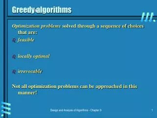
4. Greedy Method: Overview • Optimization problems: terminology • A solution must meet certain constraints: A solution is feasible • Example: All edges in solution are in graph, form a simple path • Solutions judged on some criteria: Objective function • Example: Sum of edge weights in path is smallest • One (or more) feasible solutions that scores best (by the objective function) is the optimal solution(s)

5. Greedy Method: Overview • Greedy strategy: • Build solution by stages, adding one item to partial solution found so far • At each stage, make locally optimal choice based on the greedy rule (sometimes called the selection function) • Locally optimal, i.e. best given what info we have now • Irrevocable, a choice can’t be un-done • Sequence of locally optimal choices leads to globally optimal solution (hopefully) • Must prove this for a given problem! • Approximation algorithms, heuristics

6. Proving them correct • Given a greedy algorithm, how do you show it is optimal? • As opposed to other types of algorithms (divide-and-conquer , etc.) • One common way is to compare the solution given with an optimal solution

7. Making Change

8. Making change: algorithm description • The problem: • Give back the right amount of change, and… • Return the fewest number of coins! • Inputs: the dollar-amount to return • Also, the set of possible coins. (Do we have half-dollars? That affects the answer we give.) • Output: a set of coins

9. Making change: algorithm solution • Problem description: providing coin change of a given amount in the fewest number of coins • Inputs: the dollar-amount to return. Perhaps the possible set of coins, if it is non-obvious. • Output: a set of coins that obtains the desired amount of change in the fewest number of coins • Assumptions: If the coins are not stated, then they are the standard quarter, dime, nickel, and penny. All inputs are non-negative, and dollar amounts are ignored. • Strategy: a greedy algorithm that uses the largest coins first • Description: Issue the largest coin (quarters) until the amount left is less than the amount of a quarter ($0.25). Repeat with decreasing coin sizes (dimes, nickels, pennies).

10. Making Change • Inputs: • Value N of the change to be returned • An unlimited number of coins of values d1, d2,.., dk • Output: the smallest possible set of coins that sums to N • Objective function? Smallest set • Constraints on feasible solutions? Must sum to N • Greedy rule: choose coin of largest value that is less than N - Sum(coins chosen so far) • Always optimal? Depends on set of coin values

11. Algorithm for making change • This algorithm makes change for an amount A using coins of denominations denom[1] > denom[2] > ··· > denom[n] = 1. • Input Parameters: denom, A • Output Parameters: None • greedy_coin_change(denom, A) { i = 1 while (A > 0) { c = A/denom[i] println(“use ” + c + “ coins of denomination ” + denom[i]) A = A - c * denom[i] i = i + 1 } }

12. Making change proof • Prove that the provided making change algorithm is optimal for denominations 1, 5, and 10 • Via induction, and on board -->

13. Formal proof • Formal proof of the change problem • Algorithm 7.1.1 is what is presented two slides previously

14. How would a failed proof work? • Prove that the provided making change algorithm is optimal for denominations 1, 6, and 10 • Via induction, and on board -->

15. Knapsack Algorithm

16. Knapsack Problems • Inputs: • n items, each with a weight wi and a value vi • capacity of the knapsack, C • Output: • Fractions for each of the n items, xi • Chosen to maximize total profit but not to exceed knapsack capacity

17. Two Types of Knapsack Problem • 0/1 knapsack problem • Each item is discrete. Must choose all of it or none of it. So each xi is 0 or 1 • Greedy approach does not produce optimal solutions • But another approach, dynamic programming, does • Continuous knapsack problem • Can pick up fractions of each item • The correct selection function yields a greedy algorithm that produces optimal results

18. Greedy Rule for Knapsack? • Build up a partial solution by choosing xi for one item until knapsack is full (or no more items). Which item to choose? • There are several choices. Pick one and try on this: • n = 3, C = 20 • weights = (18, 15, 10) • values = (25, 24, 15) • What answer do you get? • The optimal answer is: (0, 1, 0.5), total=31.5 • Can you verify this?

19. Possible Greedy Rules for Knapsack • Build up a partial solution by choosing xi for one item until knapsack is full (or no more items). Which item to choose? • Maybe this: take as much as possible of the remaining item that has largest value, vi • Or maybe this: take as much as possible of the remaining items that has smallest weight, wi • Neither of these produce optimal values! The one that does “combines” these two approaches. • Use ratio of profit-to-weight

20. Example Knapsack Problem • For this example: • n = 3, C = 20 • weights = (18, 15, 10) • values = (25, 24, 15) • Ratios = (25/18, 24/15, 15/10) = (1.39, 1.6, 1.5) • The optimal answer is: (0, 1, 0.5)

21. Continuous knapsack algorithm continuous_knapsack(a, C) n = a.last for i = 1 to n ratio[i] = a[i].p / a[i].w sort (a,ratio) weight = 0 i = 1 while ( i ≤ n && weight < C ) if ( weight + a[i].w ≤ C ) println (“select all of object “ + a[i].id) weight = weight + a[i].w else r = (C – weight) / a[i].w println (“select “ + r + “ of object “ + a[i].id) weight = C i++ • a is an array containing the items to be put into the knapsack. Each element has the following fields: • p: the profit for that item • w: the weight for that item • id: the identifier for that item • C is the capacity of the knapsack • What is the running time?

22. How do we know it’s correct? • Proof time!!! • On board -->

23. Prim’s MST

24. Prim’s algorithm Idea: Grow a tree by adding an edge from the “known” vertices to the “unknown” vertices. Pick the edge with the smallest weight. G v known

25. Prim’s Algorithm for MST • Pick one node as the root, • Incrementally add edges that connect a “new” vertex to the tree. • Pick the edge (u,v) where: • u is in the tree, v is not AND • where the edge weight is the smallest of all edges (where u is in the tree and v is not).

26. MST v1 {v1, v4} {v1, v2} {v4, v3} {v4, v7} {v7, v6} {v7, v5} 2 v2 v1 3 1 10 4 2 7 v3 v4 v5 8 5 4 6 v2 v1 1 v6 v7 v5 v3 v4 v7 v6

27. Minimum Spanning Tree • MSTs satisfy the optimal substructure property • If S is an optimal solution to a problem, then the components of S are optimal solutions to sub-problems • Here: an optimal tree is composed of optimal subtrees • Let T be an MST of G with an edge (u,v) in the middle • Removing (u,v) partitions T into two trees T1 and T2 • Claim: T1 is an MST of G1 = (V1,E1), and T2 is an MST of G2 = (V2,E2) • Proof: w(T) = w(u,v) + w(T1) + w(T2) • There can’t be a better tree than T1 or T2, or T would be suboptimal

28. Prim’s MST Algorithm • Greedy strategy: • Choose some start vertex as current-tree • Greedy rule: Add edge from graph to current-tree that • has the lowest weight of edges that… • have one vertex in the tree and one not in the tree. • Thus builds-up one tree by adding a new edge to it • Can this lead to an infeasible solution?(Tell me why not.) • Is it optimal? (Yes. Need a proof.)

29. Tracking Edges for Prim’s MST • Candidates edges: edge from a tree-node to a non-tree node • Since we’ll choose smallest, keep only one candidate edge for each non-tree node • But, may need to make sure we always have the smallest edge for each non-tree node • Fringe-nodes: non-trees nodes adjacent to the tree • Need data structure to hold fringe-nodes • Priority queue, ordered by min-edge weight • May need to update priorities!

30. Prim’s Algorithm MST-Prim(G, wt) init PQ to be empty; PQ.Insert(s, wt=0); parent[s] = NULL; while (PQ not empty) v = PQ.ExtractMin(); for each wadj to v if (wis unseen) { PQ.Insert(w, wt(v,w)); parent[w] = v; } else if (w is fringe && wt[v,w] < fringeWt(w)){ PQ.decreaseKey(w, wt[v,w]); parent[w] = v; }

31. Cost of Prim’s Algorithm • (Assume connected graph) • Clearly it looks at every edge, so (n+m) • Is there more? • Yes, priority queue operations • ExtractMin called n times • How expensive? Depends on the size of the PQ • descreaseKey could be called for each edge • How expensive is each call?

32. Worst Case • If all nodes connected to start, then size of PQ is n-1 right away. • Decreases by 1 for each node selected • Total cost is O(cost of extractMin for size n-1) • Note use of Big-Oh (not Big-Theta) • Could descreaseKey be called a lot? • Yes! Imagine an input that adds all nodes to the PQ at the first step, and then after that calls descreaseKey every possible time. (For you to do.)

33. Priority Queue Costs and Prim’s • Simplest choice: unordered list • PQ.ExtractMin() is just a “findMin” • Cost for one call is (n) • Total cost for all n calls is (n2) • PQ.decreaseKey() on a node finds it, changes it. • Cost for one call is (n) • But, if we can index an array by vertex number, the cost would be (1). If so, worst-case total cost is (m) • Conclusion: Easy to get (n2)

34. Better PQ Implementations • Consider using a min-heap for the Priority Queue • PQ.ExtractMin() is O(lg n) each time • Called n times, so like Heap’s Construct: efficient! • What about PQ.decreaseKey() ? • Our need: given a vertex-ID, change the value stored • But our basic heap implementation does not allow look-ups based on vertex-ID! • Solution: Indirect heaps • Heap structure stores indices to data in an array that doesn’t change • Can increase or decrease key in O(lg n) after O(1) lookup

35. Better PQ Implementations (2) • Use Indirect Heaps for the PQ • PQ.decreaseKey() is O(lg n) also • Called for each edge encountered in MST algorithm • So O(m lg n) • Overall: Might be better: (n2) than if m << n2 • Fibonacci heaps: an even more efficient PQ implementation. We won’t cover these. • (m + n lg n)

36. Kruskal’s MST

37. Kruskal’s MST Algorithm • Prim’s approach: • Build one tree. Make the one tree bigger and as good as it can be. • Kruskal’s approach • Choose the best edge possible: smallest weight • Not one tree – maintain a forest! • Each edge added will connect two trees.Can’t form a cycle in a tree! • After adding n-1 edges, you have one tree, the MST

38. Kruskal’s MST Algorithm • Idea: Grow a forest out of edges that do not create a cycle. Pick an edge with the smallest weight. G=(V,E) v

39. MST 2 v2 v1 3 1 10 4 2 7 v3 v4 v5 8 5 4 6 1 v6 v7 v2 v1 v5 v3 v4 v7 v6

40. Kruskal code void Graph::kruskal(){ intedgesAccepted = 0; DisjSet s(NUM_VERTICES); while (edgesAccepted < NUM_VERTICES – 1){ e = smallest weight edge not deleted yet; // edge e = (u, v) uset = s.find(u); vset = s.find(v); if (uset != vset){ edgesAccepted++; s.unionSets(uset, vset); } } } |E| heap ops 2|E| finds |V| unions

41. Strategy for Kruskal’s • EL = sorted set of edges ascending by weight • Foreach edge e in EL • T1 = tree for head(e) • T2 = tree for tail(e) • If (T1 != T2) • add e to the output (the MST) • Combine trees T1 and T2 • Seems simple, no? • But, how do you keep track of what trees a node is in? • Trees are sets. Need to findset(v) and “union” two sets

42. kruskal(edgelist,n) { sort(edgelist) for i = 1 to n makeset(i) count = 0 i = 1 while (count < n - 1) { if (findset(edgelist[i].v) != findset(edgelist[i].w)) { println(edgelist[i].v + “ ” + edgelist[i].w) count = count + 1 union(edgelist[i].v,edgelist[i].w) } i = i + 1 } }

43. Union/Find and Disjoint Sets • Sets stored as a parent array • findset(v): trace upward in parent array • union(i,j): make one tree a child of a node it the other • Improvements! • Union by rank • Path compression

44. Union by rank

45. Path Compression

46. Complexity for Kruskal’s • A basic analysis leads us to (n2) • But with the optimizations presented here, it can be reduced to (m lg m)

47. Interval Selection

48. Activity-Selection Problem • Problem: You and your classmates go on Semester at Sea • Many exciting activities each morning • Each starting and ending at different times • Maximize your “education” by doing as many as possible. (They’re all equally good!) • Welcome to the activity selection problem • Also called interval scheduling

49. The Activities!

50. Generalizing Start, End