Failure rates
Failure rates. outline. Failure rates as continuous distributions Weibull distribution – an example of an exponential distribution with the failure rate proportional to a power of time. The shape parameter (a) can be interpreted with respect to decreasing or increasing failure rates.

Failure rates
E N D
Presentation Transcript
outline • Failure rates as continuous distributions • Weibull distribution – an example of an exponential distribution with the failure rate proportional to a power of time. The shape parameter (a) can be interpreted with respect to decreasing or increasing failure rates. • Example problem. MWNT average lengths as a function of time. Construct the experimental failure rate curve, model with a Weibull distribution, related to reliability, hazard rate function.
Failure rates as continuous distributions Relevance to quality control, reliability testiing Mean Time Between Failures
What functions do we need?Failure rate (density function for time to 1st failure), Reliability function
Weibull distribution One example of an exponential-decaying failure rate distribution
The shape factor, a relates to change in failure rates with t
Example problem Use the MWNT fracture data in sonication experiment to generate a failure rate density function. Model this function with a Weibull distribution Interpret the coefficients with respect to rates/mechanisms
Interpretation of Weibull distribution for failure rate • We have length vs. time data for fracture of MWNTs under sonication • Failure rate for the fracture/comminution process would be the derivative of this curve. • Approach: • Fit empirical eqn. to L vs. t data • Take the derivative of this function to generate the fracture/comminuation rate (failure rate) • Model this using the Weibull distribution
Model for MWNT average lengthfailure example.xlsx. Empirical fit • Review trendline fits of power, exponential, and polynomical functions to L vs. t data. • Power law has the best R2 value, and its differential is well-behaved over the time interval
Next step.Using the best empirical fit, take the derivative, which is the fracture/failure rate for the average length particle The equation for the rate, dL/dt, can now be inserted into a moment equation – it represents f(t). When we try to fit a Weibull distribution to this model, the attempt fails. A likely problem is that our experimental distribution is not normalized.
Note: most commercial software for fitting probability density functions use normalized equations. • A pdf from raw data is not necessarily normalized. • We can use moment analysis to do this. • Sidebar: if we are after molecular weight distributions, the moment generating functions can be particularly handy for doing this Fit Weibull distribution to data
Check for normalizationMaple program. The moment is normalized if its integral over the independent variable space equals 1.0.
Normalize the distributionMaple program. Dividing the rate function by its integral values will normalize the probability density function.
Oth moment plot(moment0(t),t=1..tinf/20.);
1st moment plot(moment1(t),t=1..tinf/20);
2nd moment plot(moment2(t),t=1..tinf/20);
Weibull fit to data points Note: the Weibull distribution and this fitted function diverge significantly for t < 5 min.
Weibull cumulative distribution.Failure rate falls significantly with time; a < 1.
Alternative fitting methods for distributions We have been fitting directly to the cumulative frequency method, which does well for estimating the average. We could also minimize total error, or compare data and model across quartiles, which may be useful for regulatory actions.
Linearized lognormal.25 min data. nanocomposites design.xlsx