Maximizing Network and Storage Performance for Big Data Analytics
Maximizing Network and Storage Performance for Big Data Analytics. Xiaodong Zhang Ohio State University. Collaborators Rubao Lee, Ying Huai, Tian Luo, Yuan Yuan Ohio State University Yongqiang He and the Data Infrastructure Team, Facebook Fusheng Wang, Emory University


Maximizing Network and Storage Performance for Big Data Analytics
E N D
Presentation Transcript
Maximizing Network and Storage Performance for Big Data Analytics Xiaodong Zhang Ohio State University • Collaborators • Rubao Lee, Ying Huai, Tian Luo, Yuan YuanOhio State University • Yongqiang He and the Data Infrastructure Team, Facebook • Fusheng Wang, Emory University • Zhiwei Xu, Institute of Comp. Tech, Chinese Academy of Sciences
Digital Data Explosion in Human Society The global storage capacity Amount of digital information created and replicated in a year 2007 Analog 18.86 billion GB Analog Storage 1986 Analog 2.62 billion GB PC hard disks 123 billion GB 44.5% Digital 0.02 billion GB Digital 276.12 billion GB Digital Storage Source: Exabytes: Documenting the 'digital age' and huge growth in computing capacity, The Washington Post
Challenge of Big Data Management and Analytics (1) • Existing DB technology is not prepared for the huge volume • Until 2007, Facebook had a 15TB data warehouse by a big-DBMS-vendor • Now, ~70TB compressed data added into Facebook data warehouse every day (4x total capacity of its data warehouse in 2007) • Commercial parallel DBs rarely have 100+ nodes • Yahoo!’s Hadoop cluster has 4000+ nodes; Facebook’s data warehouse has 2750+ nodes, Google’s sorted10 PB data on a cluster of 8,000 nodes (2011) • Typical science and medical research examples: • Large Hadron Collider at CERN generates over 15 PBof data per year • Pathology Analytical Imaging Standards databases at Emory reaches 7TB, going to PB
Challenge of Big Data Management and Analytics (2) • Big data is about all kinds of data • Online services (social networks, retailers …) focus on big data of online and off-line click-stream for deep analytics • Medical imageanalytics are crucial to both biomedical research and clinical diagnosis • Complex analytics to gain deep insights from big data • Data mining • Pattern recognition • Data fusion and integration • Time series analysis • Goal: gain deep insights and new knowledge
Challenge of Big Data Management and Analytics (3) • Conventional database business model is not affordable • Expensive software license (e.g. Oracle DB, $47,500 per processor, 2010) • High maintenance fees even for open source DBs • Store and manage data in a system at least $10,000/TB* • In contrast, Hadoop-like systems only cost $1,500/TB** • Increasingly more non-profit organizations work on big data • Hospitals, bio-research institutions • Social networks, on-line services ….. • Low cost software infrastructure is a key.
Challenge of Big Data Management and Analytics (4) • Conventional parallel processing model is “scale-up” based • BSP model, CACM, 1990: optimizations in both hardware and software • Hardware: low ratio of comp/comm, fast locks, large cache and memory • Software:overlapping comp/comm, exploiting locality, co-scheduling … • Big data processing model is “scale-out” based • DOT model, SOCC’11: hardware independent software design • Scalability:maintain a sustained throughput growth by continuously adding low cost computing and storage nodes in distributed systems • Constraints in computing patterns: communication- and data-sharing-free MapReduce programming model becomes an effective data processing engine for big data analytics *: http://www.dbms2.com/2010/10/15/pricing-of-data-warehouse-appliances/ **: http://www.slideshare.net/jseidman/data-analysis-with-hadoop-and-hive-chicagodb-2212011
Why MapReduce? • A simple but effective programming model designed to process huge volumes of data concurrently • Two unique properties • Minimum dependency among tasks (almost sharing nothing) • Simple task operations in each node (low cost machines are sufficient) • Two strong merits for big data anaytics • Scalability (Amadal’s Law): increase throughput by increasing # of nodes • Fault-tolerance (quick and low cost recovery of the failures of tasks) • Hadoop is the most widely used implementation of MapReduce • in hundreds of society-dependent corporations/organizations for big data analytics: AOL, Baidu, EBay, Facebook, IBM, NY Times, Yahoo! ….
An Example of a MapReduce Job on Hadoop • Calculate average salary of each 2 organizations in a huge file. Key Value Key Value Original key/value pairs: all the person names associated with each org name and their salaries Result key/value pairs: two entries showing the org name and corresponding average salary {name: (org., salary)} {org.: avg. salary}
An Example of a MapReduce Job on Hadoop • Calculate the average salary of every organization HDFS A HDFS block Hadoop Distributed File System (HDFS) {name: (org., salary)} {org.: avg. salary}
An example of a MapReduce job on Hadoop • Calculate the average salary of every department HDFS Map Map Map Each map task takes 4 HDFS blocks as its input and extract {org.: salary} as new key/value pairs, e.g. {Alice: (org-1, 3000)} to {org-1: 3000} {name: (org., salary)} {org.: avg. salary} 3 Map tasks concurrently process input data Records of “org-1” Records of “org-2”
An example of a MapReduce job on Hadoop • Calculate the average salary of every department HDFS Map Map Map {name: (org., salary)} {org.: avg. salary} Shuffle the data using org. as Partition Key (PK) Records of “org-1” Records of “org-2”
An example of a MapReduce job on Hadoop • Calculate the average salary of every department HDFS Map Map Map Calculate the average salary for “org-2” Calculate the average salary for “org-1” {name: (org., salary)} {org.: avg. salary} Reduce (Avg.) Reduce (Avg.) HDFS
Key/Value Pairs in MapReduce • A simple but effective programming model designed to process huge volumes of data concurrently on a cluster • Map: (k1, v1) (k2, v2), e.g. (name, org & salary) (org, salary) • Reduce: (k2, v2) (k3, v3), e.g. (org, salary) (org, avg. salary) • Shuffle: Partition Key (It could be the same as k2, or not) • Partition Key: to determine how a key/value pair in the map output be transferred to a reduce task • e.g. org. name is used to partition the map output file accordingly
MR(Hadoop) Job ExecutionPatterns MR program (job) The execution of a MR job involves 6 steps Map Tasks Reduce Tasks Control level work, e.g. job scheduling and task assignment Data is stored in a Distributed File System (e.g. Hadoop Distributed File System) 1: Job submission Master node Worker nodes Worker nodes 2: Assign Tasks Do data processing work specified by Map or Reduce Function
MR(Hadoop) Job Execution Patterns MR program The execution of a MR job involves 6 steps Map Tasks Reduce Tasks 1: Job submission Map output Master node Worker nodes Worker nodes Map output will be shuffled to different reduce tasks based on Partition Keys (PKs) (usually Map output keys) 3: Map phase Concurrent tasks 4: Shuffle phase
MR(Hadoop) Job Execution Patterns MR program The execution of a MR job involves 6 steps Map Tasks Reduce Tasks 1: Job submission 6: Output will be stored back to Distributed File System Master node Worker nodes Worker nodes Reduce output 3: Map phase Concurrent tasks 5: Reduce phase Concurrent tasks 4: Shuffle phase
MR(Hadoop) Job Execution Patterns MR program The execution of a MR job involves 6 steps Map Tasks Reduce Tasks 1: Job submission 6: Output will be stored back to Distributed File System Master node Worker nodes Worker nodes A MapReduce (MR) job is resource-consuming: 1: Input data scan in the Map phase => local or remote I/Os 2: Store intermediate results of Map output => local I/Os 3: Transfer data across in the Shuffle phase => network costs 4: Store final results of this MR job => local I/Os + network costs (replicate data) Reduce output 3: Map phase Concurrent tasks 5: Reduce phase Concurrent tasks 4: Shuffle phase
Two Critical Challenges in Production Systems • Background: Conventional databases have been moved to MapReduce Environment, e.g. Hive (facebook) and Pig (Yahoo!) • Challenge 1: How to initially store the data in distributed systems • subject to minimizing network and storage cost • Challenge 2: How to automatically convert relational database queries into MapReduce jobs • subject to minimizing network and storage costs • Addressing these two Challenges, we maximize • Performance of big data analytics • Productivity of big data analytics
Challenge 1: Four Requirements of Data Placement • Data loading (L) • the overhead of writing data to distributed files system and local disks • Query processing (P) • local storage bandwidths of query processing • the amount of network transfers • Storage space utilization (S) • Data compression ratio • The convenience of applying efficient compression algorithms • Adaptive to dynamic workload patterns (W) • Additional overhead on certain queries • Objective: to design and implement a data placement structure meeting these requirements in MapReduce-based data warehouses
Initial Stores of Big Data in Distributed Environment NameNode (A part of the Master node) HDFS Blocks • HDFS (Hadoop Distributed File System) blocks are distributed • Users have a limited ability to specify customized data placement policy • e.g. to specify which blocks should be co-located • Minimizing I/O costs in local disks and intra network communication Store Block 1 Store Block 2 Store Block 3 DataNode 3 DataNode 1 DataNode 2
MR programming is not that “simple”! publicstaticclass Reduce extends Reducer<IntWritable,Text,IntWritable,Text> { private Text result = new Text(); publicvoid reduce(IntWritable key, Iterable<Text> values, Context context ) throwsIOException, InterruptedException { doublesumQuantity = 0.0; IntWritablenewKey = newIntWritable(); booleanisDiscard = true; String thisValue = new String(); intthisKey = 0; for (Text val : values) { String[] tokens = val.toString().split("\\|"); if (tokens[tokens.length - 1].compareTo("l") == 0){ sumQuantity += Double.parseDouble(tokens[0]); } elseif (tokens[tokens.length - 1].compareTo("o") == 0){ thisKey = Integer.valueOf(tokens[0]); thisValue = key.toString() + "|" + tokens[1]+"|"+tokens[2]; } else continue; } if (sumQuantity > 314){ isDiscard = false; } if (!isDiscard){ thisValue = thisValue + "|" + sumQuantity; newKey.set(thisKey); result.set(thisValue); context.write(newKey, result); } } } publicint run(String[] args) throws Exception { Configuration conf = new Configuration(); String[] otherArgs = newGenericOptionsParser(conf, args).getRemainingArgs(); if (otherArgs.length != 3) { System.err.println("Usage: Q18Job1 <orders> <lineitem> <out>"); System.exit(2); } Job job = new Job(conf, "TPC-H Q18 Job1"); job.setJarByClass(Q18Job1.class); job.setMapperClass(Map.class); job.setMapOutputKeyClass(IntWritable.class); job.setMapOutputValueClass(Text.class); job.setReducerClass(Reduce.class); job.setOutputKeyClass(IntWritable.class); job.setOutputValueClass(Text.class); FileInputFormat.addInputPath(job, new Path(otherArgs[0])); FileInputFormat.addInputPath(job, new Path(otherArgs[1])); FileOutputFormat.setOutputPath(job, new Path(otherArgs[2])); return (job.waitForCompletion(true) ? 0 : 1); } publicstaticvoid main(String[] args) throws Exception { int res = ToolRunner.run(new Configuration(), new Q18Job1(), args); System.exit(res); } } packagetpch; importjava.io.IOException; importjava.util.ArrayList; importorg.apache.hadoop.conf.Configuration; importorg.apache.hadoop.conf.Configured; importorg.apache.hadoop.fs.Path; importorg.apache.hadoop.io.DoubleWritable; importorg.apache.hadoop.io.IntWritable; importorg.apache.hadoop.io.Text; importorg.apache.hadoop.mapreduce.Job; importorg.apache.hadoop.mapreduce.Mapper; importorg.apache.hadoop.mapreduce.Reducer; importorg.apache.hadoop.mapreduce.Mapper.Context; importorg.apache.hadoop.mapreduce.lib.input.FileInputFormat; importorg.apache.hadoop.mapreduce.lib.input.FileSplit; importorg.apache.hadoop.mapreduce.lib.output.FileOutputFormat; importorg.apache.hadoop.util.GenericOptionsParser; importorg.apache.hadoop.util.Tool; importorg.apache.hadoop.util.ToolRunner; publicclass Q18Job1 extends Configured implements Tool{ publicstaticclass Map extendsMapper<Object, Text, IntWritable, Text>{ privatefinalstatic Text value = new Text(); privateIntWritable word = newIntWritable(); private String inputFile; privatebooleanisLineitem = false; @Override protectedvoid setup(Context context ) throwsIOException, InterruptedException { inputFile = ((FileSplit)context.getInputSplit()).getPath().getName(); if (inputFile.compareTo("lineitem.tbl") == 0){ isLineitem = true; } System.out.println("isLineitem:" + isLineitem + " inputFile:" + inputFile); } publicvoid map(Object key, Text line, Context context ) throwsIOException, InterruptedException { String[] tokens = (line.toString()).split("\\|"); if (isLineitem){ word.set(Integer.valueOf(tokens[0])); value.set(tokens[4] + "|l"); context.write(word, value); } else{ word.set(Integer.valueOf(tokens[0])); value.set(tokens[1] + "|" + tokens[4]+"|"+tokens[3]+"|o"); context.write(word, value); } } } This complex code is for a simple MR job Low Productivity! We all want to simply write: “SELECT * FROM Book WHERE price > 100.00”?
Challenge 2: High Quality MapReduce in Automation A job description in SQL-like declarative language A interface between users and MR programs (jobs) SQL-to-MapReduce Translator Write MR programs (jobs) MR programs (jobs) Workers Hadoop Distributed File System (HDFS)
Challenge 2: High Quality MapReduce in Automation A job description in SQL-like declarative language A interface between users and MR programs (jobs) SQL-to-MapReduce Translator Write MR programs (jobs) • Improve productivity from hand-coding MapReduce programs • 95%+Hadoop jobs in Facebook are generated by Hive • 75%+ Hadoop jobs in Yahoo! are invoked by Pig* A MR program (job) A data warehousing system (Facebook) A high-level programming environment (Yahoo!) Workers Hadoop Distributed File System (HDFS) * http://hadooplondon.eventbrite.com/
Outline • RCFile: a fast and space-efficient placement structure • Re-examination of existing structures • A Mathematical model as the analytical basis for RCFile • Experiment results • Ysmart: a high efficient query-to-MapReduce translator • Correlations-aware is the key • Fundamental Rules in the translation process • Experiment results • Impact of RCFile and Ysmart in production systems • Conclusion
Row-Store: Merits/Limits with MapReduce Table • Data loading is fast (no additional processing); • All columns of a data row are located in the same HDFS block • Not all columns are used (unnecessary storage bandwidth) • Compression of different types may add additional overhead
Distributed Row-Store Data among Nodes HDFS Blocks NameNode Store Block 1 Store Block 2 Store Block 3 DataNode 3 DataNode 1 DataNode 2
Column-Store: Merits/Limits with MapReduce Column group 1 Column group 2 Column group 3 • Unnecessary I/O costs can be avoided: • Only needed columns are loaded, and easy compression • Additional network transfers for column grouping
Distributed Column-Store Data among Nodes HDFS Blocks NameNode Store Block 1 Store Block 2 Store Block 3 DataNode 3 DataNode 1 DataNode 2
Optimization of Data Placement Structure • Consider the four requirements comprehensively • The optimization problem becomes: • In an environment of dynamic workload (W) and with a suitable data compression algorithm (S) to improve the utilization of data storage, find a data placement structure (DPS) that minimizes the processing time of a basic operation (OP) on a table (T) with ncolumns • Two basic operations • Write: the essential operation of data loading (L) • Read: the essential operation of query processing (P)
Write Operations Table • Load the table into HDFS blocks based on • different data placement structure • HDFS blocks are distributed to Datanodes HDFS Blocks DataNode 3 DataNode 1 DataNode 2
Read Operation in Row-store • Read local rows concurrently ; • Discard unneeded columns HDFS Blocks DataNode 3 DataNode 1 DataNode 2
Read Operations in Column-store Project A&C Project C&D Transfer them to a common place via networks DataNode 3 DataNode 3 DataNode 1
An Expected Value based Statistical Model • In probability theory, the expected value of an random variable is • Weighted average of all possible values of this random variable can take on • Estimated big data access time can take time of “read” T(r) and “write” T(w), each with a probability (p(r) and p(w)) since p(r) + p(w) = 1, and read and write have equal weights, estimated access time is a weighted average: • E[T] = p(r) * T(r) + p(w) * T(w)
Overview of the Optimization Model processing time of a read operation processing time of a write operation Probabilities of write and read operations
Overview of the Optimization Model The majority of operation is read, so ωr>>ωw ~70TB of compressed data added per day and PB level compressed data scanned per day in Facebook (90%+) We focus on minimization of processing time of read operations
Modeling Processing Time of a Read Operation • # of combinations of n columns a query needs is up to
Modeling Processing Time of a Read Operation • # of combinations of n columns a query needs is up to • Processing Time of a Read Operation
Expected Time of a Read Operation n: the number of columns of table T i: i columns are needed j: it is jth column combination in all combinations with i columns
Expected Time of a Read Operation The frequency of occurrence of jth column combination in all combinations with i columns. We fix it as a constant value to represent a environment with highly dynamic workload
Expected Time of a Read Operation The frequency of occurrence of jth column combination in all combinations with i columns. We fix the probability as a constant value to represent a environment with highly dynamic workload
Expected Time of a Read Operation The time used to read needed columns from local disks in parallel S: The size of the compressed table. We assume with efficient data compression algorithms and configurations, different DPSs can achieve comparable compression ratio Blocal: The bandwidth of local disks ρ: the degree of parallelism, i.e. total number of concurrent nodes
Expected Time of a Read Operation α(DPS): Read efficiency. % of columns read from local disks Only read necessary columns Read all columns, including unnecessary columns
Expected Time of a Read Operation The extra time on network transfer for row construction
Expected Time of a Read Operation The extra time on network transfer for row construction λ(DPS, i, j, n): Communication Overhead. Additional network transfers for row constructions
Expected Time of a Read Operation The extra time on network transfer for row construction λ(DPS, i, j, n): Communication Overhead. Additional network transfers for row constructions All needed columns are in one node (0 communication) At least two columns are in two different nodes
Expected Time of a Read Operation The extra time on network transfer for row construction λ(DPS, i, j, n): Communication Overhead. Additional network transfers for row constructions All needed columns are in one node (0 communication) Transferring data via networks β:% of data transferred via networks (DPS, workload dependent), 0%≤β≤100%
Expected Time of a Read Operation The extra time on network transfer for row construction Bnetwork: The bandwidth of the network
Finding Optimal Data Placement Structure Can we find a Data Placement Structure with both optimal read efficiency and communication overhead ?
Goals of RCFile • Eliminate unnecessary I/O costs like Column-store • Only read needed columns from disks • Eliminate network costs in row construction like Row-store • Keep the fast data loading speed of Row-store • Can apply efficient data compression algorithms conveniently like Column-store • Eliminate all the limits of Row-store and Column-store