Games with Secure Equilibria
Games with Secure Equilibria . Krishnendu Chatterjee (Berkeley) Thomas A. Henzinger (EPFL) Marcin Jurdzinski (Warwick). Classification of 2-Player Games. Zero-sum games: complementary payoffs. Non-zero-sum games: arbitrary payoffs. 1,-1. 0,0. 3,1. 1,0. -1,1. 2,-2. 3,2. 4,2.

Games with Secure Equilibria
E N D
Presentation Transcript
Games with Secure Equilibria Krishnendu Chatterjee (Berkeley) Thomas A. Henzinger (EPFL) Marcin Jurdzinski (Warwick)
Classification of 2-Player Games • Zero-sum games: complementary payoffs. • Non-zero-sum games: arbitrary payoffs. 1,-1 0,0 3,1 1,0 -1,1 2,-2 3,2 4,2
Classical Notion of Rationality Nash equilibrium: none of the players gains by deviation. 3,1 1,0 (row, column) 3,2 4,2
Classical Notion of Rationality Nash equilibrium: none of the players gains by deviation. 3,1 1,0 (row, column) 3,2 4,2
New Notion of Rationality Nash equilibrium: none of the players gains by deviation. Secure equilibrium: none hurts the opponent by deviation. 3,1 1,0 (row, column) 3,2 4,2
Secure Equilibria • Natural notion of rationality for component systems: • First, a component tries to meet its spec. • Second, a component may obstruct the other components. • For -regular specs, there is always unique maximal secure equilibrium.
Games on Graphs • Modeling component interaction: • Vertices = states • Players = components • Moves = transitions • Applications: • Synthesis (control) of sequential systems • Verification of adversarial specs • Receptiveness • Compatibility • Early error detection • (Bi)simulation checking • Model checking • Game semantics • etc.
Example: Verification Starvation Freedom (mutual exclusion protocols, cache coherence protocols) In a multi-process system, can a process that wishes P to proceed always eventually proceed no matter what the other processes do? 8(a )hhPii} b) 8 (a )8} b) X 8 (a !9} b) X
Example: Verification Starvation Freedom (mutual exclusion protocols, cache coherence protocols) In a multi-process system, can a process P that wishes to proceed always eventually proceed no matter what the other processes do provided they meet their specs ? 8(a )hhPii } b) X 8 (a )8} b) X 8 (a !9} b) X
Games on Graphs • Turn-based (perfect-information) games: • Game graph G=((V,E), (V1,V2)). • E µ V £ V: serial edge relation. • (V1,V2): partition of the vertex set V. • The game is played by moving token along edges of the graph: • V1: player-1 moves the token. • V2: player-2 moves the token.
Example: A Game Graph s3 s0 s1 s2
Plays and Strategies • Play (outcome) of a game: • Infinite path (s0,s1,…) of states si 2 V such that (si,si+1) 2 E for all i ¸ 0. • : set of all plays. • Player-1 strategy: • Given prefix of play ending in V1, specifies how to extend the play. • : V*¢ V1! V such that (s, (x¢s)) 2 E for all x 2 V* and s 2 V1. • Symmetric definition for player-2 strategies . • Given two strategies , and a start state s, there is a unique play , (s).
Example s3 s0 s1 s2 • Example of a play: s0 s1 s2 • Strategies that yield this play: • - Player-1: s0! s1 • - Player-2: s1! s2
Memoryless Strategies • Independent of the history of the play: : V1! V : V2! V • Yield simple controllers. • Existence puts games into NP.
Objectives and Payoffs • What the players are playing for: • Player-1 objective: play in set 1µ V . • Player-2 objective: play in set 2µ V . • General objectives: Borel sets in the Cantor topology. • Finite-state objectives: -regular sets (level 2.5 Borel sets). • From objectives to payoffs: • If , (s) 2i , then player i gets payoff 1 else payoff 0. • The payoff profile for a strategy profile (,) at a state s is (v1, (s), v2, (s)).
Classification of Games • Zero-sum games: • Complementary objectives: 2 = :1. • Possible payoff profiles (1,0) and (0,1). • Non-zero-sum games: • Arbitrary objectives 1, 2. • Possible payoff profiles (1,1), (1,0), (0,1), and (0,0).
Zero-Sum Games on Graphs • Winning: -Winning-1 states s: (9) (8) ,(s) 2 1. - Winning-2 states s: (9) (8) ,(s) 2 2. • Determinacy: • Every state is winning-1 or winning-2. • Borel determinacy [Martin 75]. • Memoryless determinacy for parity games [Emerson/Jutla 91]. (1,0) (0,1)
Non-Zero-Sum Games on Graphs Nash equilibrium (,) at state s: (8’) v1, (s) ¸ v1’, (s) (8 ’) v2, (s) ¸ v2,’ (s)
Example: Reachability Game R2 R1 s3 s0 s1 s2 Objective for player i is to visit Ri.
Example R2 R1 s3 s0 s1 s2 Nash equilibria: (s0! s1, s1! s2): (1,0)
Example R2 R1 s3 s0 s1 s2 Nash equilibria: (s0! s1, s1! s2): (1,0) (s0! s3, s1! s0): (0,1) (s0! s1, s1! s0): (0,0)
Example R2 R1 s3 s0 s1 s2 Nash equilibria: (s0! s1, s1! s2): (1,0) (s0! s3, s1! s0): (0,1)
-Regular Objectives Synthesis: - Zero-sum game controller versus plant. - Control against all plant behaviors. Verification: - Non-zero-sum specs for components. - Components may behave adversarially, but without threatening their own specs.
Non-Zero-Sum Verification Games Drawbacks of Nash equilibrium: - Does not capture adversarial behavior. - Not unique. A new notion of equilibrium: - Takes into account both non-zero-sum payoffs and adversarial behavior. - Captures the essence of component-based systems. - Unique for Borel objectives. - Computable for -regular objectives.
Secure Equilibria • Secure strategy profile (,) at state s: (8’) ( v1,’ (s) < v1, (s) ) v2,’ (s) < v2, (s) ) (8’) ( v2’, (s) < v2, (s) ) v1’, (s) < v1, (s) ) • A secure profile (,) is a contract: if the player-1 deviates to lower player-2’s payoff, her own payoff decreases as well, and vice versa. • Secure equilibrium: secure strategy profile that is also a Nash equilibrium.
Secure Equilibria 3,3 1,3 2,1 0,0 3,1 2,2 0,0 1,2 (row, column)
Example R2 R1 s3 s0 s1 s2 Nash equilibria: (s0! s1, s1! s2): (1,0) (s0! s3, s1! s0): (0,1) (s0! s1, s1! s0): (0,0) not secure
Example R2 R1 s3 s0 s1 s2 Nash equilibria: (s0! s1, s1! s2): (1,0) (s0! s3, s1! s0): (0,1) (s0! s1, s1! s0): (0,0) not secure not secure
Example R2 R1 s3 s0 s1 s2 Nash equilibria: (s0! s1, s1! s2): (1,0) (s0! s3, s1! s0): (0,1) (s0! s1, s1! s0): (0,0) not secure not secure secure
Lexicographic Payoff Profile Ordering • Player-1 preference º1 : • (v1,v2) Â1 (v’1,v’2) iff v1 > v’1 or ( v1 = v’1 and v2 < v’2 ). • (v1,v2) º1 (v’1,v’2) iff (v1,v2) Â1 (v’1,v’2) or (v1,v2) = (v’1,v’2). • Player-2 preference º2 symmetric. • Captures payoff maximization with external adversarial choice. • Provides notion of maximality: • Player-1: (1,0) º1 (1,1) º1 (0,0) º1 (0,1) • Player-2: (0,1) º2 (1,1) º2 (0,0) º2 (1,0)
Alternative Characterization A secure equilibrium is an equilibrium with respect to the º1 and º2 payoff profile orderings: A strategy profile (,) is a secure equilibrium at s iff (8’) (v1, (s), v2, (s)) º1 (v1’, (s), v2’, (s)) (8’) (v1, (s), v2,’ (s)) º2 (v1,’ (s), v2,’ (s))
Example: Buechi Game B1 s1 s3 s2 s0 B2 s4 Objective for player i is to visit Bi infinitely often.
Example B1 s1 s3 s2 s0 B2 s4 Nash equilibria: (s0! s4, s1! s4): (0,0) secure
Example B1 s1 s3 s2 s0 B2 s4 Nash equilibria: (s0! s4, s1! s4): (0,0) (s0! s1, s1! s0): (1,0) secure
Example B1 s1 s3 s2 s0 B2 s4 Nash equilibria: (s0! s4, s1! s4): (0,0) (s0! s1, s1! s0): (1,0) secure not secure
Example B1 s1 s3 s2 s0 B2 s4 Nash equilibria: (s0! s4, s1! s4): (0,0) (s0! s1, s1! s0): (1,0) (s0! s2, s3! s1): (1,1) secure not secure
Example B1 s1 s3 s2 s0 B2 s4 Nash equilibria: (s0! s4, s1! s4): (0,0) (s0! s1, s1! s0): (1,0) (s0! s2, s3! s1): (1,1) secure not secure
Example B1 s1 s3 s2 s0 B2 s4 Nash equilibria: (s0! s4, s1! s4): (0,0) (s0! s1, s1! s0): (1,0) (s0! s2, s3! s1): (1,1) secure not secure secure
Example B1 s1 s3 s2 s0 B2 s4 • Secure equilibrium (,) with payoff (1,1) at s0: • : if s1! s0, then s2 else s4. : if s3! s1, then s0 else s4. • Pair of “retaliating” strategies. • Require memory.
Maximal Secure Equilibria Theorem: At every state s of a graph game with Borel objectives, there is a unique secure equilibrium profile that is maximal with respect to both º1 and º2. This is the rational behavior of both players at s if they wish to 1. satisfy their own objectives and, then, 2. sabotage the opponent’s objective.
Strongly Winning and Retaliating Strategies • Winning strategies: • Player-1 wins for the objective 1. • Player-2 wins for 2. • Strongly winning strategies: • Player-1 wins for the objective 1Æ:2. • Player-2 wins for 2Æ:1. • Retaliating strategies: • Player-1 wins for the objective 2)1. • Player-2 wins for 1)2.
Winning Sets • W1: set of states s.t. player-1 has a winning strategy. • W2: set of states s.t. player-2 has a winning strategy. • W10: set of states s.t. player-1 has a strongly winning strategy. • W01: set of states s.t. player-2 has a strongly winning strategy. • W11: set of states s s.t. there is a pair (,) of retaliating strategies with ,(s) ²1Æ2. • W00: set of states s s.t. each player has a retaliating strategy and for every pair (,) of retaliating strategies, ,(s) ²:1Æ:2.
State Space Partition hh2ii ( :1Ç2 ) W10 hh1ii ( 1Æ:2 )
State Space Partition W01 hh2ii ( 2Æ:1 ) hh2ii ( :1Ç2 ) hh1ii ( :2Ç1 ) W10 hh1ii ( 1Æ:2 )
State Space Partition W01 hh2ii ( 2Æ:1 ) hh2ii ( :1Ç2 ) Retaliating strategies hh1ii ( :2Ç1 ) W10 hh1ii ( 1Æ:2 ) There is no player-2 retaliating strategy in W10, and no player-1 retaliating strategy in W01.
Retaliating Strategy Pairs • Every player-1 retaliating strategy ensures for every player-2 strategy that 2)1. • Hence every pair (,) of retaliating strategies ensures (:1Ç:2) ) (:1Æ:2). • W11 and W00are the regions of the state space where both players have retaliating strategies: • W11 contains the states where some pair (,) of retaliating strategies ensures 1Æ2. • W00 contains the states where all pairs (,) of retaliating strategies lead to :1Æ:2.
State Space Partition W00 W01 hh2ii ( 2Æ:1 ) W10 hh1ii ( 1Æ:2 ) W11
Uniqueness of Maximal Secure Equilibria W11: (1,1) is a secure equilibrium, and hence maximal W10: (1,0) is the only secure equilibrium W01: (0,1) is the only secure equilibrium W00: (0,0) is the only possible secure equilibrium W11 is the set of states where both players can collaborate to win, yet each player keeps an “insurance policy.”
Generalization of Determinacy Zero-sum games:2 = :1 Non-zero-sum games:1, 2 W1 W00 W01 W11 W2 W10