Interactive Auditory Display
Interactive Auditory Display. Ming C. Lin Department of Computer Science University of Maryland at College Park lin@cs.umd.edu http:// gamma.cs.umd.edu /Sound. How can it be done?. Foley artists manually make and record the sound from the real-world interaction. Lucasfilm Foley Artist.


Interactive Auditory Display
E N D
Presentation Transcript
Interactive Auditory Display Ming C. Lin Department of Computer Science University of Maryland at College Park lin@cs.umd.edu http://gamma.cs.umd.edu/Sound
How can it be done? • Foley artists manually make and record the sound from the real-world interaction Lucasfilm Foley Artist
How about Computer Simulation? • Physical simulation drives visual simulation • Sound rendering can also be automaticallygenerated via 3D physical interaction
Sound Rendering: An Overview Scientific Visualization Specular Reflection Late Reverberation Acoustic Geometry -- surface simplification Scattering Personalized HRTFs for 3D sound Diffraction Acoustic Material -- absorption coefficient -- scattering coefficient Refraction Digital Signal Processing Doppler Effect Source Modeling -- area source -- emitting characteristics -- sound signal Interpolation for Dynamic Scenes Attenuation Interference 3D Audio Rendering Modeling Propagation
Low geometric detail vs. High geometric detail Modeling Acoustic vs. Graphics Acoustic Geometry -- surface simplification Acoustic Material -- absorption coefficient -- scattering coefficient Source Modeling -- area source -- emitting characteristics -- sound signal Modeling
343 m/s vs.300,000,000 m/s 20 to 20K Hzvs. RGB 17m to 17cm vs.700 to 400 nm Propagation Acoustic vs. Graphics Specular Reflection Scattering Diffraction Refraction Doppler Effect Attenuation Interference Propagation
Compute intensive DSP vs. addition of colors 44.1 KHz vs. 30 Hz Psychoacoustics vs. Visual psychophysics 3D Audio Rendering Acoustic vs. Graphics Late Reverberation Personalized HRTFs for 3D sound Digital Signal Processing Interpolation for Dynamic Scenes 3D Audio Rendering
Modeling Acoustic Geometry [Vorländer,2007] Visual Geometry Acoustic Geometry
Modeling Sound Material [Embrechts,2001] [Christensen,2005] [Tsingos,2007]
Modeling Sound Source Volumetric Sound Source Directional Sound Source Complex Vibration Source
Advanced Interfaces Multi-sensory Visualization Applications Minority Report (2002) Multi-variate Data Visualization
Games VR Training Applications Medical Personnel Training Game (Half-Life 2)
Acoustic Prototyping Applications Symphony Hall, Boston Level Editor, Half Life
Strict time budget for audio simulations Games are dynamic Moving sound sources Moving listeners Moving scene geometry Trade-off speed with the accuracy of the simulation Static environment effects (assigned to regions in the scene) Sound Propagation in Games
Main Components 3D Audio and HRTF Artifact free rendering for dynamic scenes Handling many sound sources 3D Audio Rendering
Perceptual Audio Rendering [Moeck,2007] Multi-Resolution Sound Rendering [Wand,2004] 3D Audio Rendering
Overview of Sound Simulation • The complete pipeline for sound simulation • Sound Synthesis • Sound Propagation • Sound Rendering
Overview of Sound Simulation • Sound Synthesis
Overview of Sound Simulation • Sound Propagation
Overview of Sound Simulation • Sound Rendering
Our System Set-up Tablet Support User Interface
Main Results • An interactive and flexible work flow for sound synthesis • User control over material parameters • Intuitive interaction and real-time auditory feedback for easy testing and prototyping • No event synchronization issue: users with little or no foley experience can start sound design and creation quickly • Easy integration with game engines
Main Results [Ren et al; VR 2010] • A new frictional contact model for sound synthesis • Fast, allows real-time interaction • Simulates frictional interactions at different levels: • Macro shape • Meso bumpiness • Micro roughness • Better matches their virtually-simulated visual counterparts
System Overview • Sound synthesis module • Modal Analysis: Raghuvanshi & Lin (I3D 2006) • Impulse response
System Overview • Interaction handling module • State detection: lasting and transient contacts • Converting interactions into impulses
Modal Analysis • Deformation modeling • Vibration of surface generates sound • Sound sampling rate: 44100 Hz • Impossible to calculate the displacement of the surface at sampling rate • Represent the vibration pattern by a bank of damped oscillators (modes) • Standard technique for real-time sound synthesis
Modal Analysis • Discretization • An input triangle mesh a spring-mass system • A spring-mass system a set of decoupled modes
Modal Analysis • The spring-mass system set-up • Each vertex is considered as a mass particle • Each edge is considered as a damped spring
Modal Analysis • Coupled spring-mass system to a set of decoupled modes
Modal Analysis • A discretized physics system • We use spring-mass system • Small displacement, so consider it linear Stiffness Damping Mass Stiffness Damping Mass
Modal Analysis • Rayleigh damping And diagonalizing • Solve the Ordinary Differential Equation (ODE) • Now, solve this ODE instead
Modal Analysis • Substitute (z are the modes) Now, solve this ODE instead • Solve the ODE
Modal Analysis • General solution • External excitation defines the initial conditions
Modal Analysis • Assumptions • In most graphics applications, only surface representations of geometries are given • A surface representation is used in modal Analysis • Synthesized sound appears to be “hallow”
Modal Analysis Summary • An input triangle mesh A spring-mass system A set of decoupled modes
State Detection • Distinguishing between lasting and transient contacts • In contacts? • In lasting contacts?
Interaction Handling • Lasting contacts a sequence of impulses • Transient contacts a single impulse
Impulse Response • Dirac Delta function as impulse excitation • General solution • with initial condition given by the impulse, • we have:
Handling Lasting Contacts • i.e. Frictional contacts • How to add the sequence of impulses? • The model has to be fast and simple, because…
Handling Lasting Contacts Update Rate: 100Hz Update Rate: 44100Hz
Handling Lasting Contacts • The interaction simulation has to be stepped at the audio sampling rate: 44100 Hz • The update rate of a typical real-time physics simulator: on the order of 100’s Hz • Not enough simulation is provided by the physics engine • An customized interaction model for sound synthesis
Our Solution • Decompose the interaction into difference levels • Different update rates at different levels • Combined results offer a good approximation
Our Solution • Three levels of simulation • Macro level: simulating the interactions on the overall surface shape • Meso level: simulating the interactions on the surface material bumpiness • Micro level: simulating the interactions on the surface material roughness
Three-level Simulation • Macro level: Geometry information • Update rate: 100’s Hz • Update rate does not need to be high • The geometry information is from the input triangle mesh, and contacts are reported by collision detection in the physics engine.
Three-level Simulation • Meso level: Bumpiness • Bump mapping is ubiquitous in real-time graphics rendering • Bump maps are visible to users but transparent to physics simulation
What Is Bump Mapping? • Perturb vertex normals for shading • No geometry details • + = Image Courtesy to Wikipedia
Three-level Simulation • Meso level simulation • Makes sure visual and auditory cues are consistent • Attends to surface bumpiness details • Update rate: • Event queue: 100’sHz • Event processor: 44100 Hz