Automatic Performance Tuning of Numerical Kernels: BeBOP for Optimized Computing
840 likes | 963 Vues
This report presents the BeBOP project focusing on automatic performance tuning of numerical kernels, primarily for dense and sparse matrix operations. Led by James Demmel and Katherine Yelick from UC Berkeley with support from NSF and DOE, the project aims to improve the performance of applications heavily reliant on specific computational kernels. The findings include tuning strategies, recent results on various architectures, and future work proposals. Contributions come from faculty, researchers, and students involved in shaping advanced tuning methodologies in numerical computing.

Automatic Performance Tuning of Numerical Kernels: BeBOP for Optimized Computing
E N D
Presentation Transcript
Automatic Performance Tuningof Numerical Kernels BeBOP: Berkeley Benchmarking and OPtimization James Demmel EECS and Math UC Berkeley Katherine Yelick EECS UC Berkeley Support from NSF, DOE SciDAC, Intel
Performance Tuning Participants • Other Faculty • Michael Jordan, William Kahan, Zhaojun Bai (UCD) • Researchers • Mark Adams (SNL), David Bailey (LBL), Parry Husbands (LBL), Xiaoye Li (LBL), Lenny Oliker (LBL) • PhD Students • Rich Vuduc, Yozo Hida, Geoff Pike • Undergrads • Brian Gaeke , Jen Hsu, Shoaib Kamil, Suh Kang, Hyun Kim, Gina Lee, Jaeseop Lee, Michael de Lorimier, Jin Moon, Randy Shoopman, Brandon Thompson
Outline • Motivation, History, Related work • Tuning Dense Matrix Operations • Tuning Sparse Matrix Operations • Results on Sun Ultra 1/170 • Recent results on P4 • Recent results on Itanium • Future Work
Performance Tuning • Motivation: performance of many applications dominated by a few kernels • CAD Nonlinear ODEs Nonlinear equations Linear equations Matrix multiply • Matrix-by-matrix or matrix-by-vector • Dense or Sparse • Information retrieval by LSI Compress term-document matrix … Sparse mat-vec multiply • Many other examples (not all linear algebra)
Conventional Performance Tuning • Motivation: performance of many applications dominated by a few kernels • Vendor or user hand tunes kernels • Drawbacks: • Very time consuming and tedious work • Even with intimate knowledge of architecture and compiler, performance hard to predict • Growing list of kernels to tune • Example: New BLAS (Basic Linear Algebra Subroutines) Standard • Must be redone for every architecture, compiler • Compiler technology often lags architecture • Not just a compiler problem: • Best algorithm may depend on input, so some tuning at run-time. • Not all algorithms semantically or mathematically equivalent
Automatic Performance Tuning • Approach: for each kernel • Identify and generate a space of algorithms • Search for the fastest one, by running them • What is a space of algorithms? • Depending on kernel and input, may vary • instruction mix and order • memory access patterns • data structures • mathematical formulation • When do we search? • Once per kernel and architecture • At compile time • At run time • All of the above
Some Automatic Tuning Projects • PHIPAC (www.icsi.berkeley.edu/~bilmes/phipac) (Bilmes,Asanovic,Vuduc,Demmel) • ATLAS (www.netlib.org/atlas) (Dongarra, Whaley; in Matlab) • XBLAS (www.nersc.gov/~xiaoye/XBLAS) (Demmel, X. Li) • Sparsity (www.cs.berkeley.edu/~yelick/sparsity) (Yelick, Im) • FFTs and Signal Processing • FFTW (www.fftw.org) • Won 1999 Wilkinson Prize for Numerical Software • SPIRAL (www.ece.cmu.edu/~spiral) • Extensions to other transforms, DSPs • UHFFT • Extensions to higher dimension, parallelism • Special session at ICCS 2001 • Organized by Yelick and Demmel • www.ucalgary.ca/iccs • Proceedings available • Pointers to other automatic tuning projects at • www.cs.berkeley.edu/~yelick/iccs-tune
Tuning Techniques in PHIPAC • Multi-level tiling (cache, registers) • Copy optimization • Removing false dependencies • Exploiting multiple registers • Minimizing pointer updates • Loop unrolling • Software pipelining • Exposing independent operations • Copy optimization
Untiled (“Naïve”) n x n Matrix Multiply Assume two levels of memory: fast and slow for i = 1 to n {read row i of A into fast memory} for j = 1 to n {read C(i,j) into fast memory} for k = 1 to n {read B(k,j) into fast memory} C(i,j) = C(i,j) + A(i,k) * B(k,j) {write C(i,j) back to slow memory} A(i,:) C(i,j) C(i,j) B(:,j) = + *
Untiled (“Naïve”) n x n Matrix Multiply - Analysis Assume two levels of memory: fast and slow for i = 1 to n {read row i of A into fast memory} for j = 1 to n {read C(i,j) into fast memory} for k = 1 to n {read B(k,j) into fast memory} C(i,j) = C(i,j) + A(i,k) * B(k,j) {write C(i,j) back to slow memory} Count Number of slow memory references m = n3 to read each column of B n times + n2 to read each row of A once for each i + 2n2 to read and write each element of C once = n3 + 3n2
Tiled (Blocked) Matrix Multiply Consider A,B,C to be N by N matrices of b by b subblocks where b=n / N is called the block size for i = 1 to N for j = 1 to N {read block C(i,j) into fast memory} for k = 1 to N {read block A(i,k) into fast memory} {read block B(k,j) into fast memory} C(i,j) = C(i,j) + A(i,k) * B(k,j) {do a matrix multiply on blocks} {write block C(i,j) back to slow memory} A(i,k) C(i,j) C(i,j) = + * B(k,j)
Tiled (Blocked) Matrix Multiply - Analysis • Why is this algorithm correct? • Number of slow memory references on blocked matrix multiply m = N*n2 to read each block of B N3 times (N3 * n/N * n/N) + N*n2 to read each block of A N3 times + 2n2 to read and write each block of C once = (2N + 2) * n2 ~ (2/b) * n3 • b = n/N times fewer slow memory references than untiled algorithm • Assumes all three bxb blocks from A,B,C must fit in fast memory • 3b2 <= M = fast memory size • Decrease in slow memory references limited to a factor of O(sqrt(M)) • Theorem (Hong & Kung, 1981): “Any” reorganization of this algorithm (using only associativity) has at least O(n3/sqrt(M)) slow memory refs • Apply tiling recursively for multiple levels of memory hierarchy
PHIPAC: Copy optimization • Copy input operands • Reduce cache conflicts • Constant array offsets for fixed size blocks • Expose page-level locality Original matrix, column major (numbers are addresses) Reorganized into 2x2 blocks 0 4 8 12 0 2 8 10 1 5 9 13 1 3 9 11 2 6 10 14 4 6 12 13 3 7 11 15 5 7 14 15
PHIPAC: Removing False Dependencies • Using local variables, reorder operations to remove false dependencies a[i] = b[i] + c; a[i+1] = b[i+1] * d; false read-after-write hazard between a[i] and b[i+1] float f1 = b[i]; float f2 = b[i+1]; a[i] = f1 + c; a[i+1] = f2 * d; • With some compilers, you can say explicitly (via flag or pragma) that a and b are not aliased.
PHIPAC: Exploiting Multiple Registers • Reduce demands on memory bandwidth by pre-loading into local variables while( … ) { *res++ = filter[0]*signal[0] + filter[1]*signal[1] + filter[2]*signal[2]; signal++; } Before float f0 = filter[0]; float f1 = filter[1]; float f2 = filter[2]; while( … ) { *res++ = f0*signal[0] + f1*signal[1] + f2*signal[2]; signal++; } also: register float f0 = …; After
PHIPAC: Minimizing Pointer Updates • Replace pointer updates for strided memory addressing with constant array offsets f0 = *r8; r8 += 4; f1 = *r8; r8 += 4; f2 = *r8; r8 += 4; f0 = r8[0]; f1 = r8[4]; f2 = r8[8]; r8 += 12;
PHIPAC: Loop Unrolling • Expose instruction-level parallelism float f0 = filter[0], f1 = filter[1], f2 = filter[2]; float s0 = signal[0], s1 = signal[1], s2 = signal[2]; *res++ = f0*s0 + f1*s1 + f2*s2; do { signal += 3; s0 = signal[0]; res[0] = f0*s1 + f1*s2 + f2*s0; s1 = signal[1]; res[1] = f0*s2 + f1*s0 + f2*s1; s2 = signal[2]; res[2] = f0*s0 + f1*s1 + f2*s2; res += 3; } while( … );
Load(i) Load(i+1) Load(i+2) Mult(i) Mult(i+1) Mult(i+2) Add(i) Add(i+1) Add(i+2) PHIPAC: Software Pipelining of Loops • Mix instructions from different iterations • Keeps functional units “busy” • Reduce stalls from dependent instructions i i+1 i+2 i Load(i+2) Mult(i+1) Add(i) i+1 Load(i+3) Mult(i+2) Add(i+1) Load(i+4) Mult(i+3) Add(i+2) i+2
PHIPAC: Exposing Independent Operations • Hide instruction latency • Use local variables to expose independent operations that can execute in parallel or in a pipelined fashion • Balance the instruction mix (what functional units are available?) f1 = f5 * f9; f2 = f6 + f10; f3 = f7 * f11; f4 = f8 + f12;
Tuning pays off – ATLAS (Dongarra, Whaley) Extends applicability of PHIPAC Incorporated in Matlab (with rest of LAPACK)
Search for optimal register tile sizes on Sun Ultra 10 16 registers, but 2-by-3 tile size fastest
Search for Optimal L0 block size in dense matmul 4% of versions exceed 60% of peak on Pentium II-300
High Precision Algorithms (XBLAS) • Double-double (High precision word represented as pair of doubles) • Many variations on these algorithms; we currently use Bailey’s • Exploiting Extra-wide Registers • Suppose s(1) , … , s(n) have f-bit fractions, SUM has F>f bit fraction • Consider following algorithm for S = Si=1,n s(i) • Sort so that |s(1)| |s(2)| … |s(n)| • SUM = 0, for i = 1 to n SUM = SUM + s(i), end for, sum = SUM • Theorem (D., Hida) Suppose F<2f (less than double precision) • If n 2F-f + 1, then error 1.5 ulps • If n = 2F-f + 2, then error 22f-F ulps (can be 1) • If n 2F-f + 3, then error can be arbitrary (S 0 but sum = 0 ) • Examples • s(i) double (f=53), SUM double extended (F=64) • accurate if n 211 + 1 = 2049 • Dot product of single precision x(i) and y(i) • s(i) = x(i)*y(i) (f=2*24=48), SUM double extended (F=64) • accurate if n 216 + 1 = 65537
Tuning pays off – FFTW (Frigo, Johnson) Tuning ideas applied to signal processing (DFT) Also incorporated in Matlab
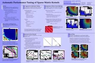
Tuning Sparse matrix-vector multiply • Sparsity • Optimizes y = A*x for a particular sparse A • Im and Yelick • Algorithm space • Different code organization, instruction mixes • Different register blockings (change data structure and fill of A) • Different cache blocking • Different number of columns of x • Different matrix orderings • Software and papers available • www.cs.berkeley.edu/~yelick/sparsity
How Sparsity tunes y = A*x • Register Blocking • Store matrix as dense r x c blocks • Precompute performance in Mflops of dense A*x for various register block sizes r x c • Given A, sample it to estimate Fill if A blocked for varying r x c • Choose r x c to minimize estimated running time Fill/Mflops • Store explicit zeros in dense r x c blocks, unroll • Cache Blocking • Useful when source vector x enormous • Store matrix as sparse 2k x 2l blocks • Search over 2k x 2l cache blocks to find fastest
Register-Blocked Performance of SPMV on Dense Matrices (up to 12x12) 333 MHz Sun Ultra IIi 800 MHz Pentium III 70 Mflops 175 Mflops 35 Mflops 105 Mflops 1.5 GHz Pentium 4 800 MHz Itanium 425 Mflops 250 Mflops 310 Mflops 110 Mflops
Which other sparse operations can we tune? • General matrix-vector multiply A*x • Possibly many vectors x • Symmetric matrix-vector multiply A*x • Solve a triangular system of equations T-1*x • y = AT*A*x • Kernel of Information Retrieval via LSI (SVD) • Same number of memory references as A*x • y = Si (A(i,:))T * (A(i,:) * x) • Future work • A2*x, Ak*x • Kernel of Information Retrieval used by Google • Includes Jacobi, SOR, … • Changes calling algorithm • AT*M*A • Matrix triple product • Used in multigrid solver • What does SciDAC need?
Test Matrices • General Sparse Matrices • Up to n=76K, nnz = 3.21M • From many application areas • 1 – Dense • 2 to 17 - FEM • 18 to 39 - assorted • 41 to 44 – linear programming • 45 - LSI • Symmetric Matrices • Subset of General Matrices • 1 – Dense • 2 to 8 - FEM • 9 to 13 - assorted • Lower Triangular Matrices • Obtained by running SuperLU on subset of General Sparse Matrices • 1 – Dense • 2 – 13 – FEM • Details on test matrices at end of talk