Spatial Databases - Indexing
Spatial Databases - Indexing. Spring, 2010 Ki-Joune Li. What is Indexing ?. Indexing : Fight against TIME Example Suppose that you have a Hamlet , and you want to know the name of Hamlet’s father. Without Index : Full (Sequential) Scan of the book With Index : Direct Access to the Page.


Spatial Databases - Indexing
E N D
Presentation Transcript
Spatial Databases- Indexing Spring, 2010 Ki-Joune Li
What is Indexing ? • Indexing : Fight against TIME • Example Suppose that you have a Hamlet, and you want to know the name of Hamlet’s father. • Without Index : Full (Sequential) Scan of the book • With Index : Direct Access to the Page Hamlet
Some Constraints • Modern Database • Very Huge Volume : e.g. several peta bytes • Storage on Disk • Inevitable • But slow (cf. main memory) : msec. vs. nano sec. • Even in Main Memory Database System • What should we do ? Minimize the number of Disk Access
Disk Address (Block Number) Index Indexing The Objective of Indexing Database in Disk Query Condition
Disk Address (Block Number) Spatial Index Spatial predicate Classification of Indexing • According to the type of query and data • Alphanumeric query • Image • Spatial • What is the nearest post office to the Louvre Museum ? Database in Disk Spatial Query
Spatial Query • Sophisticated • Types of Spatial Query • One Scan Query • Region Query : Containment, Intersection • K-Nearest Neighbor Query • Multi-Scan Query : Join • Spatial Join • Distance Join • Spatial Query Processing • Tightly coupled with Spatial Indexing Method
Verification of Geometry Candidates Result Simplification of Geometry Complete Data 1. More Light Index : e.g. < 1 M bytes 2. Remove Unnecessary Disk Accesses Spatial Processing Strategy • Filtering and Refinement Strategy Index Spatial Query Filtering Refinement
Classification of Spatial Indexing Methods • Hashing and Indexing • Index (in wide sense) • Hashing, Indexing (in narrow sense) • Space Decomposition vs. MBR • Decomposition of a space : Whole Space • Bounding Rectangle : Only Interesting Area • Dimensionality • No Transformation • to Higher Dimension • To Lower Dimension : Linearization
Indexing vs. Hashing • Hashing • 1. b = h(r.key) • 2. Store(r, b) • Block number is determined by hashing function or mechanism • Only for primary index • Search by a hashing function • Indexing (in narrow sense) • 1. b = Store(r ) • 2. Insert(B, (r.key, b) ) • Block number is independent from indexing mechanism • For primary or secondary index • Search by a data structure called index
Decomposition Bounding Region Decomposition vs. Bounding Region
Decomposition Methods • Grid File : An Extension of Hashing to 2-D • Variation • Fixed Grid • Grid File • Multi-Level Grid File • Hierarchical Data Structure • KD-tree • Quadtree • skd-tree • etc.
1 Disk Page Query Window 40 30 20 10 0 0 10 20 30 40 50 Fixed Grid • Most Simple Method • Minimum Data for Hashing 1. Find intersecting grids 2. Find corresponding blocks 3. Read objects from the blocks 4. Refinement
Query Window 40 30 20 10 0 0 10 20 30 40 50 Problems of Fixed Grid • Only for Point Object • Object with measure : duplicated storage • Degrade performance • Large Dead Space • Causes Unnecessary Disk Accesses • Not very Flexible • On Distribution
Grid Boundary Block# A (0,0),(15,20) Page 0 B (15,0),(30,20) Page 1 . . . . . . . . . Directory Query Window I (30,28),(50,40) Page 15 Grid File • To overcome problems of Fixed Grid • Reduce Dead Space within a cell • Increase Blocking Factor 40 28 20 0 0 15 20 30 50
Blocking Factor • A Key Factor on performance • Number of Objects in a Disk Block • Number of Disk Accesses • How to increase Bf ? • Increase Block Size : not always possible • Packing
Grid Boundary Block# A (0,0),(15,20) Page 0 B (15,0),(30,20) Page 1 . . . . . . . . . Directory I (30,28),(50,40) Page 15 Problems of Fixed Grid • Only for Point Object • Still Large Dead Space • Large Size of Directory
Hierarchical Decomposition • To overcome the size of directory in Grid File • Hierarchical Structure of Directory • Acceleration of Search
A Directory x=20 =< < y=10 y=20 x=30 Each leaf node points to the disk page KD-tree : Index • Extension of Binary Tree to K-Dimension (K=2 for us) • Example : suppose Bf =3 B E 15 A E B 10 D A C C D 30 20
KD-tree : Search B E x=20 =< < y=10 y=20 15 x=30 A A E B 10 D A C C D 30 20
Weak Points of KD-tree • Only for Point Objects • Dead Space • How to Store Tree Structure on Disk Space • Blocking Problem • Widely used for main memory index • Rarely used for disk resident index • Unbalanced Tree • Zipf’s Law (or 80/20 law) • Most events are concentrated • Leads highly skewed tree B E D A C
Each leaf node points to the disk page Quadtree • Extension of KD-tree : • KD-tree : binary split • Quadtree 4-way equi-split instead • Example : Bf =3 C D F A F B E B C D E G H I J H J G A I
Weak Points of Quadtree • Same Problems of KD-tree • In addition to the lack of flexibility • Only for Point Objects • Dead Space • How to Store Tree Structure on Disk Space • Blocking Problem • Widely used for main memory index • Rarely used for disk resident index • Unbalanced Tree • Zipf’s Law (or 80/20 law) • Most events are concentrated • Leads highly skewed tree
Point Quadtree • A Simple Variation of Quadtree • Specification of Partition Point instead of equi-split • More Adaptive to the distribution of objects • Less Skewed (10,20) (5,25) A (5,25) F (35,10) (10,20) B C D E G H I J (35,10)
6 13 11 Linear Quadtree : Space-Filling Curve • Quadtree but another representation • Linearization by Space-Filling Curve Hilbert Column-wise N-order Linearize points(or cells) by their peano-key
Peano key = 1 0 0 1 Linear Quadtree • Example : N-order curve • Computation of Peano-Key : Bit-Interleaving 11 1. Binary representation of coordinates (10,01) 2. Bit-Interleaving x = 1 0 y = 0 1 10 01 00 = 9 00 01 10 11
(X1max, X2max ) (X1min, X2min) MBR Methods • MBR (Minimum Bounding Box) • Two dimensional geometric simplification of objects • Not the Whole space, • only in the region occupied by objects • R-tree and its variants
H I B C D E F G J K R-tree • Construction of R-tree : Sequence of Insertion • Upward Split R-tree B C E A H F G I D J K A Leaf node points to the disk page 2-D Objects
New MBR Splitting in R-tree • Split MBR in the case of overflow • Line sweeping : Compare Cost-X and Cost-Y Splitting Line • Cost Measure • Area, • Perimeter • Overlapping Area
C F G A B C D E F G J A H I B I H D E K K J Candidate Query Region W R-tree : Query Processing B C E H F I G D J K A Read its exact geometry from databaseCandidate Refinement Sample : http://www.dbnet.ece.ntua.gr/~mario/rtree/
B E C E H F I G D J D K A C Strength of R-tree • For point and non-point Objects • Good for non-uniform distribution • Paged Tree • Hierarchical Structure but Balanced • Less Dead Space than Decomposition Methods
M K J L G D A H E B I F C Query Region Weak Points of R-tree : Overlapping Area • Overlapping : False Matching A B G C L H J K D I K E F M False Matching : Visit unnecessary node Performance Degradation
Query Region Weak Points of R-tree : Dead Space A B G C L H J D I E K F M At least one visit at this node (K) even though there is nothing
Good Split Bad Split Weak Points of R-tree : Bad Split • 50:50 Split 1. Make them as COMPACT as possible 2. Preserve spatial proximity as possible
Improvement of R-tree • Minimize • Overlapping area • Dead Space • Or Make it more COMPACT • Preserve Spatial Proximity • Two approaches • Packing (or Bulk Loading) • Good Split or Insertion Strategies
Newly Inserted Object Delete and Re-Insert this R*-tree : An Improvement of R-tree • Re-Insertion Strategy on Overflow Overflow
More Compact Re-Inserted Object R*-tree : An Improvement of R-tree • Re-Insertion Strategy on Overflow
R*-tree : An Improvement of R-tree • R*-tree • Compact • Small Overlapping Area • Small Sum of MBR area or perimeters • Small Dead Space • Stable : Not very affected by the order of insertions • The most widely used spatial indexing method
Packing R-tree : Improvement of R-tree • Preprocessing for making R-tree more compact • Hilbert R-tree • STR (Sort-Tile Recursive) • Uniformization • Instead of Sequential Insertions
Hilbert Packing • Hilbert Curve • A Space Filling Curve • Linearize spatial objects by their peano-key N-order Hilbert Column-wise
Hilbert Packing • Hilbert Packing • Sort objects by Hilbert key • Packing by round-robin way • Maximize storage utilization • Minimum Dead Space, and Sum of MBR area • Example: Bf =3
STR (Sort-Tile Recursive) • Basic idea : “tile” the data space using vertical slices • r : number of rectangles • n : blocking factor • P ( leaf node page ) = Example Suppose r = 25, n =3 nTile = 9, nV = 3, nH = 3
Large Objects Points Comparison : Hilbert Packing vs. STR HP STR HP STR
Uniformization • Non-Uniform Distribution • Negative Effect on the performance • But in real applications : Non-Uniform • Uniformization Technique • Step 1 : Transform Non-Uniform data to Uniform by STR • Step 2 : Apply R-tree (or Fixed Grid) • Step 3 : Transform Query Region • Strength • High Storage Utilization • Very Simple and Good Performance
Uniformization Equi-Width Non Equi-Width 1. Area of each cell : identical2. Number of objects within each cell : almost identical
Uniformization : Example By Delaunay Triangulation By STR Original
Uniformization : Example Original By STR
Query Point Query Processing by R-tree : Nearest Neighbor Searching Space 2nd Distances in 2-D Minimum
Query Processing by R-tree : Nearest Neighbor Branching Branching Pruning Minimum
Transformation to Higher Space • Transformation to Higher Dimension • Transform non-point object to point object • Reuse of spatial indexing methods (e.g. Grid File) applicable only to point objects to non-point objects • Example Max C B B A A C Amin Amax Min
Corner Transformation • From 2-D to 4-D 1. Simplification by MBR 2. MBR ((Xmin, Ymin), (Xmax, Ymax)) to Point (Xmin, Ymin, Xmax, Ymax) (Xmax, Ymax) (Xmin, Ymin)