Chapter 3. Several Random Variables
Chapter 3. Several Random Variables. # How to extend the probabilistic description of a single random variable to include the more realistic situation of continuous time functions? # As the first step, consider two random variables. - this can be extended to an infinite # of rv’s

Chapter 3. Several Random Variables
E N D
Presentation Transcript
Chapter 3. Several Random Variables # How to extend the probabilistic description of a single random variable to include the more realistic situation of continuous time functions? # As the first step, consider two random variables. - this can be extended to an infinite # of rv’s - there are some cases where only two rv’s are involved
If the random variables associated with any two instants of time can be described, then all of the information is available to carry out most of system analysis. There are many situations where only two rv’s are involved. For example, suppose that we are interested in finding the I/O relation of the system either at the same time instant or at two different time instants.
3.1 Two Random Variables # To deal with two random variables, it is necessary to extend the concepts of pdf & PDF. - Definition : joint PDF & pdf of two random variables X & Y
Properties of joint PDF • Properties of joint pdf
Examples tossing two coins
A pair of random variables having a density function that is constant between x1 and x2 and between y1 and y2
# The joint pdf can be used to find the expected value of functions of two random variables in the same way as with the single variable density function. (Remark) When , the expected value is known as the correlation given by
Consider the example of a pair of random variables “marginal pdf”
3.2 Conditional Probability - Revisited Now, consider the case where the event M depends on some other random variable Y.
There are several different ways where the given event M can be defined in terms of Y. Case 1: M is the event Case 2: M is the event
The most common form of conditional probabilityis one where M is the event that Y=y. (Note) In almost all these case Pr(M)=0 Let and and by taking The conditional pdf is given by
Conditional Probability Density Function or - the continuous version of Bayes’ theorem - another expression of the marginal pdf
The joint probability density function completely specifies both marginal density functions and both conditional density functions. As an illustrative example, consider a joint pdf of the form -Integrating this wrt y alone and wrt x alone gives the two marginal pdf - Now, the two conditional pdf are written as
Now, we will consider one of the most common and typical applications of the conditional density function, that is, the estimation problem. Suppose a signal X(t) is perturbed by additive noise N(t) where are assumed known. The problem is to find the conditional pdf of X, given the observed value of Y.
따라서 와 은 알려져 있다고 가정하였으므로 “a priori pdf”, 를 구할 수 있음. 그러면 일때 optimal estimate 은 을 최대로 하는 x이다.
Then 오직 의 최대점의 위치만 알고 싶으면( for a given Y, simply a constant)
의 exponent만을 고려 ▶ exponent가 minimum 일 때 는 최대 ▶ exponent를 x에 관하여 미분
Two case 즉 일 때 즉 일 때 P 129 그림 3.3 참조
3.3 Statistical Independence # When two random variables are statistically independent, a knowledge of one random variable gives no information about the value of the other. # Definition(statistical independence) : - Some consequences of statistical independence
3.4 Correlation of two random variables # Whether one random variable depends in any way on another random variable? # Definition: ; covariance ;correlation coefficient or normalized covariance
ρ의 성질 Check by yourself If X and Y are statistically indep. ρ = 0 하지만, ρ = 0 이라고 해서 statistically indep. 한것도 아니다. (단, Gaussian r.v. 에 대해서는 성립)
Two random variables jointly gaussian When ρ = 0, -> statistically indep.
Recall that • 의 Variance는? ……………………. Uncorrelated ρ = 0이면 결과일치!
3.5 Density Function of Z = X + Y ( assumption: two rv are statistically independent) Since Y it can be obtained as follows X+Y=z X
Therefore, pdf of Z is simply the convolution of pdf of X & Y Similarly, we can obtain another form from
( Example ) 1 1 1 1 0.632 1
What will happen if the two rv are independent & gaussian? The sum of the two independent Gaussian random variables is Gaussian with a mean that is the sum of means and a variance that is the sum of the variances. reproducible property
# What will happen if the two Gaussian rv is correlated ? The answer is still Gaussian with # In summary, Gaussian Gaussian Linear System r.v. everywhere Gaussian Sinusoidal Sinusoidal Linear System Freq w Freq w
# pdf of the sum of two rv smoother pdf Convolution # pdf of the sum of more rv much smoother pdf Converge toward Gaussian pdf “Central Limit Theorem” See example in pp. 140 -141
3.6 pdf of a fu. of two r.v.’s new two r.v.’s inversely
그런데 y w 영역대응 dzdw dxdy x z
절대값 By coordinate transformation 여기서 J 는 자코비안 (Jacobian) 따라서
예) 예) X,Y는 statistically indep. uniformly distributed
99.5< z <100.5 • 그런데 z의 범위는 9.952(99.0025)에서 10.052(101.0025) 문제) Z=XY 면적에 관한 r.v, nominal 값은 100㎠±0.5% 내에 들어갈 확률은? pdf of z
그런데 z의 범위는 9.952< z <10.052이를 구분 i) 9.952< z <9.95ⅹ10.05=99.9975 ii) 9.95ⅹ10.05< z <10.052 왜냐면 9.95< w < 10.05 인데, (z/10.05)< w <(z/9.95) 이므로 i)의 경우는 9.952< z <9.95ⅹ10.05 9.95< w <(z/9.95) ii)의 경우는 9.95ⅹ10.05< z <10.052 (z/10.05)< w < 10.05
따라서 교재 p.146 그림 3.8 참조
3.7 The Characteristic Function Two indep. r.v’s의 sum → convolution • Convolution의 Fourier transform은 multiplication이라는 점에 착안 (r.v.’s 수가 늘어남에 따라 repeated convolution은 tedious)
② Applications : ①
② finding the correlation H.W : Solve the problems; 3-1.2, 3-2.2, 3-3.1, 3-4.1, 3-5.1, 3-5.5 3-6.1, 3-7.1, 3-7.5