Download
1 / 71
760 likes | 1.26k Vues
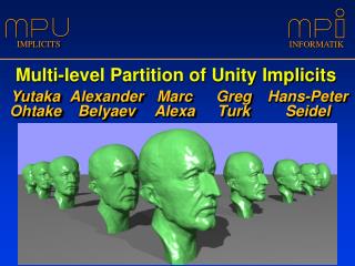
Siggraph 2004. Yutaka Ohtake, Alexander Bylyaev, Marc Alexa, Greg Turk, Hans-Peter Seidel. Multi-level partition of unity implicits. Abstract. We present a new shape representation , the multi-level partition of unity implicit surface.

E N D
Siggraph 2004 Yutaka Ohtake, Alexander Bylyaev, Marc Alexa, Greg Turk, Hans-Peter Seidel Multi-level partition of unity implicits
Abstract • We present a new shape representation, • the multi-level partition of unity implicit • surface. - Very large sets of points 으로 부터 surface를 construct. • Three key ingredients • Quadratic function : capture the local shape of the surface. • Weighting functions(partitions of unity) the blend together these local shape functions. • Octree subdivision method.
Abstract • Represent sharp feature (edges, corners) • Time, memory 소비는 depends on the • requried accurary • Local approximation과 local blending을 분리하였기 때문에, global 하지 않고, 빠르게 수행된다. • Implicit surface를 사용했기 때문에, shape • blending, offsets, deformation, CSG
Introduction Touch Probes Laser Range Finder Depth from stereo로 object를 디지털화 한다. 이런 기술들은 millionsof 3d point를 추출한다.
Introduction • 노이즈, mis-registration이 발생했을때, interpolation하는 것보다는 approximation 하는 것이 낫다. • 적절하게 sharp feature 를 reproduction. • Hole이 있는 부분에서도 robust.
Introduction Goal : Representing implicit solid as a function f Input : Points with Normals
Introduction 이 논문에서는, large collections of point으로 부터 정확한 surface를 만들어 낸다. We use the name Multi-level Partition of Unity (MPU) , 왜냐하면, 이 메소드의 핵심은 set of weight function이기 때문이다. Set of points MPU는 surface로 부터signed distance 로 approximatin할 수 있다.
Introduction Approximation은 surface에 가까울수록정확하다. Surface는 distance function의 zero level set에 의해서 approximated.
Introduction 우리는 point들 ( )이 노말 ( ) 을가지고 있다고 가정한다. 특히, 노말들은 의 local least-squares에 의해서나, shape acquisition phase 동안에 초기 scans으로 부터 얻을 수 있다. 우리는 mesh에 대해서도 surface가 근사화될때를 가정하고, 은mesh vertices의 집합, 은 mesh vertex의 normal이다.
Introduction To create our implicit representation, 우리는 먼저 point set에 대한 bounds를 설정하고, 이 bouding box로 octree based subdivision을 한다. • 각 octree cell에 대한 quadratic function(the • local shape function)은 cell 내부에 있는 • points에 적합하게 만들어 진다. • 그들의 shape function은 대체로 signed distance와 같게 실행이 된다.
Introduction Data points 근처에서는 0, 내부는 positive를, 외부는 negative를 얻게 될 것이다. 점들의 근사 노말은 지역적으로 in/out side를 구분하는데 사용된다. Shape function의 근사화가 not accurate enough(포인트들이 잘 math가 되는 않는다면), 그 cell은 subdivide and procedure is repeated until a certain accuracy is achieved.
Introduction Octree Level에 따른, local shape complexity와 desired accuracy의 관계를 보여주고 있다.
Introduction 2개 혹은 그 이상의 cells의 공통 boundary에서는 shape function은 Partition of unity function으로 부터의 weight 에 따라서 blend 될 것이다.
Introduction global implicit function of surface는 octree leafs에서의 local shape 근사화의 blending에 의해서 주어진다. Octree Node Leaf Node
Introduction MPU은 scattered point data로 부터 adaptive 하게 복잡한 shape을 빠르고 정확하게 reconstruction 한다. Creation time, memory 소비는 shape reconstruction의 complexity에 의존한다.
Previouswork Implicit surface는 복잡한 모델을 쉽게 묘사 할수 있고, shape editing을 쉽게 수행할 수 있다. Introduction to Implicit Surfaces [Bloomenthal 1997] 흩어진 포인트들로 부터 shape reconstruction을 하기위해, implicit surface를 사용하는 것에 대한 장점은 repairing능력과 editing할수 있는 능력이다.
Previouswork Point sets으로 부터 implicit shape 복구의 기반이 되는 기술은 Blinn’s idea of blending local implicit primitives. A generalization of Algebraic Surface Drawing [Blinn 1982] Point set으로 부터 implicit surface를 fit 하기 위해서 Gaussian Linear combimation을 사용했다 Volumetric Shape Description of Range Data using “Blobby Model”[Blinn 1982]
Previouswork locally estimate the signed distance function as the distance to the tangent plane of the closest point. Surface Reconstruction from Unorganized Points [Hoppe et al 1992] 흩어진 포인트로 부터 implicit surface를 reconstruction 하기위해서 use blended union of spheres. Implicit Reconstruction of Solids from Cloud Point Sets [Lim et al. 1995]
Previouswork Range scan으로 부터 shape 을 reconstruction 하는 것이다. A volumetric method for building complex models from range images [Curless and Levoy et al 1996] Interpolating Implicit Surfaces From Scattered Surface Data Using Compactly Supported Radial Basis Functions. [Savchenko et al 1995] Reconstruction and representation of 3D object with radial basis functions. [Carr et al 2001] Modeling with implicit surfaces that interpolate. [Truk, O’Brien 2002] Globally Radial Basis Function 기반
Previouswork Function representation of solids reconstructed from scattered surface points and contours. [Morse et al. 2001] Software Tools Using CSRBFs for Processing Scattered Data. [Kojekine et al. 2003] A Multi-scale Approach to 3D Scattered Data Interpolation with Compactly Supported Basis Functions. [Ohtake et al. 2003] Compactly supported Radial Basis Function 기반
Previouswork Level set mthod는 reconstructingsigned distance field 기 위한 또 다른 좋은 방법이다. [Zhao and Osher 2002] 그러나 high accuracy에 대해서는 expensive. Shape을 근사화 하기 위한 Projection-based approaches은 local(point수에 독립적), 직접적으로 surface의 point를 추출한다. [Alexa at al. 2000; Fleishman et al 2003] 그러나 MSL(non linear problem)을 사용하기 때문에 이거 또한 expensive.
Previouswork 우리의 기술은 몇몇 알고 있는 blend 기술들과 유사하다. RBF method는 data domain을 몇 개의 cells로 나눈다. 그래서 data는 다루기 쉬운 조각으로 나누어 진다. [Beatson, et al 2000; Schaback and Wendland 2000; Iske 2001;Iske and Levesley 2002; Wendland 2002] domain을 decomposition에서 1980년 Franke and Nielson에 의해 제안된 partition of unity(PU)는 일반적인 FEM method에서 사용되어져 왔다.
Previouswork 최근에 그것은 mesh를 construct 할 때, topological Overhead를 피하기 위해서 많이 사용되었다. [Babuska and Melenk 1997; Griebel and Schweitzer 2000; Griebel and Schweitzer 2002] 최근 우리의 MPU는 adaptively sampled distance field [Frisken et al.2000]이랑 비슷하다.
Previouswork 우리의 local shape approximation을 적절한게 선택해서, 사용을 했을 때, 아래와 같은 장점을 가질 수 있다. • Very large point datasets으로 부터 높은 질의 mesh를 만들 수 있다. • Sharp feature를 정확하게 표현 할 수 있고, 빠르고, 쉽게 local shape을 access 할 수 있다.
Partition of Unity Approach • Partition of unity approach는 전형적으로 locally 하게 global 근사화안에서 정의된다. • Maximum error 와 수렴 차수 local behavior로 부터 수렴된다. • Partition of unity 의 기본아이디어는 • Domain을 몇몇 조각으로 나눈다. • 각 subdomain 에서 데이터를 근사화 한다. • Smooth , local한 weight를 이용해서 local solution을 blend
Partition of Unity Approach Local approximation function은 V(i)의 집합. f(x) 의 approximation은 다음과 같이 정의. Partition of unity function 다음과 같이 정의.
Partition of Unity Approach Local approximation Q(x)는 “inverse distance” Singular weights {w(x)}와 combination되어서 사용되어 진다. Inverse distance?? 측정된 값은 포인트들의 주변 강도, 거리의 함수이다. Inverse distance weight는 포인트들의 거리에 대한 영향력의 감쇠 정도를 나타냄. 가까이 있는 값에 더 큰 가중 값을 주어 보간 하는방법.
Partition of Unity Approach W : 가중치 = 1/d (d : v와 v’사이의 거리) I : 영향 범위 내에 해당하는 샘플점 Z : 추정치(neighbor of v)
Partition of Unity Approach • Octree-based adaptive space subdivision. • : error of the approximation 을 조절. • : shape의 복잡도를 표현할 수 있다. • 2. Shape feature를 정확하게 표현하기 위해 • Boolean operator로부 터 나온 Piecewise Quadratic function을 사용한다. • 우리는 approximation을 위해, quadratic B- • spline b(t)를 사용한다.
Partition of Unity Approach w(i) is defined as a circle of radius r(i), centered on the middle of the node(i). C(i) : center of the node(i) in the octree. 우리는 inverse distance weight를 사용~!! [Franke and Nielson 1980; Renka 1988]
Adaptive Octree-based Approximation d : length of the diagonal of the cell c : center of the cell 우리는 R을 정의한다. 알파가 커지면, better (smoother) 보간, 근사화된다. 결과적으로 computation time이 더 걸리게 된다.
Adaptive Octree-based Approximation Zero level set으로부터 떨어진 distance 함수의 approximation의 정확도 를 표현한 것이다. 1-4개의 모델은 알파=0.75이다. 마지막 모 델은 알파=1을사용했다. quality가 높다.
Adaptive Octree-based Approximation cell은 subdivision되는 동안에 generated 된다. Local shape function Q(x)는 least Squares fitting에 의해서 만들어 진다.
Adaptive Octree-based Approximation Density of points가 uniform하지 않다면, 즉, R에 포함되는 point가 충분하지 않다면 R을 증가시켜준다. N(min) = 15 는 local shape function Q(x)를 계산 하는데 사용한다.
Adaptive Octree-based Approximation epsilon 이 epsilon(0) 보다 크다면, subdivide. Leaf-node만 계산. 다른 local approximation을 사용한다.(near, far) 이것은 Coarse approximation에 대한 보정없이, Sharp feature approximation 나타냄. Coarse approximation 을 피하는 것은 memory 를 절약 하고, implicit function의 평가를 더 빠 르게 한다.
Estimating Local Shape Functions Local fittingfunction은 주어진 cell의 ball내에 있는 points의 개수와 노말요소에 의존적이다. 3개의 근사화 함수에서 가장 적절한 한 개를 사용을 한다. (1) Surface의 넓은 부분을 근사화 한다. (2) Local smooth patch를 근사화 한다. (3) Sharp feature를 reconstruction 한다.
Estimating Local Shape Functions (3) 은 surface approximation의 타입을 결정하기 위해서 하는 edge & corner test 이다. [Feature sensitive surface extraction from valume data. Kobbelt et al] Local ball내에 있는 points가 2N(min)보다 많다 면, (1) 또는 (2)을 실행한다. 평균 노말에서 가장 큰 노말의 변화량이 파이/2 보다 크다면 (1)를 실행그렇지 않다면 (2)를 실행
Estimating Local Shape Functions 왜? 2N(min)보다 많은 곳에서만 sharp Features를 찾는가???????? Sharp features는 computation complexity한 곳에서 발견되고, octree subdivision은 이걸 중요시 한다. Cell 에서 corner or edge가 포함되었다면, 그때, Quality-of-fit 를 계산해서, cell을 divide할지를 결정. Sharp feature는 한 개 또는 그 이상의 cell에 의해서 Fit 이 될 것이다.
Estimating Local Shape Functions c : center of subdivision cubic cell. p‘ : point of inside the ball of the cell. n : unit normal vector 에 의해 계산된 weight와 p’의 평균노말의 노말라이즈. theta : n와 p’의 normal과에 가장 큰 각도 theta >= Pi/2 Theta < Pi/2
Local Shape Function (Qi) • Least square fitting. • Approximation type : according to the • Deviation of normals. Local fit of a bivariate quadratic polynomial Local fit of a general quadric
(a) Local fit of a general quadric If |p’| > 2N(min) && theta >= Pi/2 Local shape function A, b, c를 결정하기 위해서, 보조 포인트(auxiliary)를 사용한다. 이것은 local shape function의 방향 결정을 도와준다.
(a) Local fit of a general quadric • 보조 포인트(auxiliary){qi} • 분할된 cell의 각 코너와 중심 • 보조 포인트는 믿을 수 있는 • Signed distance 값인지 아닌지 • 를 판별한다. • 각 q는 6개의 neighbor p(1)…p(6)을 가진다. p(i)는 p’ • 로 부터 가장 가까운 neighbor point 이다. 평면의 벡터 방정식