Two Level and Multi level Minimization
Two Level and Multi level Minimization. Espresso Algorithm. 1. Expands implicants to their maximum size Implicants covered by an expanded implicant are removed from further consideration Quality of result depends on order of implicant expansion

Two Level and Multi level Minimization
E N D
Presentation Transcript
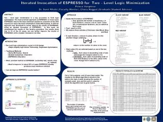
Espresso Algorithm 1. Expands implicants to their maximum size Implicants covered by an expanded implicant are removed from further consideration Quality of result depends on order of implicant expansion Heuristic methods used to determine order Step is called EXPAND Irredundant cover (i.e., no proper subset is also a cover) is extracted from the expanded primes Just like the Quine-McCluskey Prime Implicant Chart Step is called IRREDUNDANT COVER Solution usually pretty good, but sometimes can be improved Might exist another cover with fewer terms or fewer literals Shrink prime implicants to smallest size that still covers ON-set Step is called REDUCE Repeat sequence REDUCE/EXPAND/IRREDUNDANT COVER to find alternative prime implicants Keep doing this as long as new covers improve on last solution A number of optimizations are tried, e.g., identify and remove essential primes early in the process 2. 3. 4. 5.
Details of ESPRESSO Algorithm Procedure ESPRESSO ( F, D, R) /* F is ON set, D is don’t care, R OFF * R = COMPLEMENT(F+D); /* Compute complement */ F = EXPAND(F, R) ; /* Initial expansion */ F = IRREDUNDANT(F,D); /* Initial irredundant cover */ F = ESSENTIAL(F,D) /* Detecting essential primes */ F = F - E; /* Remove essential primes from F */ D = D + E; /* Add essential primes to D */ WHILE Cost(F) keeps decreasing DO F = REDUCE(F,D); /* Perform reduction, heuristic which cubes */ F = EXPAND(F,R); /* Perform expansion, heuristic which cubes */ F = IRREDUNDANT(F,D); /* Perform irredundant cover */ ENDWHILE; F = F + E; RETURN F; END Procedure;
Need for Iterations in ESPRESSO Espresso: Why Iterate on Reduce, Irredundant Cover, Expand? Initial Set of Primes found by Steps1 and 2 of the Espresso Method Result of REDUCE: Shrink primes while still covering the ON-set Choice of order in which to perform shrink is important 4 primes, irredundant cover, but not a minimal cover!
ESPRESSO Example Espresso Iteration (Continued) IRREDUNDANT COVER found by final step of espresso Only three prime implicants! Second EXPAND generates a different set of prime implicants
Example of ESPRESSO Input/Output ƒ(A,B,C,D) = m(4,5,6,8,9,10,13) + d(0,7,15) Espresso Input Espresso Output -- # inputs -- # outputs -- input names -- output name -- number of product terms -- A'BC'D' -- A'BC'D -- A'BCD' -- AB'C'D' -- AB'C'D -- AB'CD' -- ABC'D -- A'B'C'D' don't care -- A'BCD don't care -- ABCD don't care -- end of list .i 4 .o 1 .ilb a b c d .ob f .p 3 1-01 1 10-0 1 01-- 1 .e .i 4 .o 1 .ilb a b c d .ob f .p 10 0100 1 0101 1 0110 1 1000 1 1001 1 1010 1 1101 1 0000 - 0111 - 1111 - .e ƒ = A C' D + A B' D' + A' B
Espresso :: conclusion • The algorithm successively generates new covers until no further improvement is possible. • Produces near-optimal solutions. • Used for PLA minimization, or as a sub-function in multilevel logic minimization. • Can process very large circuits. • 10,000 literals, 100 inputs, 100 outputs • Less than 15 minutes on a high-speed workstation
Multilevel Logic Minimization • In many applications, 2-level logic is unsuitable as compared to random (multilevel) logic. • Gates with high fanin are slow, and take more area. • It makes sense to transform a 2-level logic realization to multi-level logic.
A classical example :: XOR function • For an 8-input XOR function, • For 2-level NAND-NAND realization 8C1 + 8C3 + 8C5 + 8C7 = 128 NAND8 gates 1 NAND128 gate • For 3-level XOR realization 7 XOR2 gates 28 NAND2 gates Number of levels = 9
Multilevel logic optimization: • Local • Rule-based transformation • Global • Weak division
Local Optimization Technique • Used in IBM Logic Synthesis System. • Perform rule-based local transformations. • Objective reduce area, delay, power. • Developing a good set of rules is a challenge. • Should be comprehensive enough so as to completely explore the design space. • Basic idea: • Apply a transformation which reduces cost. • Iterate and continue the transformations as long as solution keeps improving.
AND/OR transformations • Reduce the size of the circuit, critical path. • Typical transformations: a . 1 = a a + 1 = 1 a + a’ = 1 a . a’ = 0 (a’)’ = a a + a’ . b = a + b xor (xor(a1,a2,…,an), b) = xor (a1,a2,…,an,b) • Transform the AND/OR form to NAND form (or NOR form).
NAND (NOR) transformations • Some synthesis systems assume that all gates are of the same type (NAND or NOR). • Does not require technology mapping. • Rules framed that transform a NAND (NOR) network to another. • Examples: NAND (NOT (NAND (a,b)), c) = NAND (a,b,c) NAND (NAND(a,b,c), NAND(a,b,c’)) = NAND(a,b)
How complex is the algorithm? • n number of circuit nodes m number of rules • Ordering of rule (by cost reduction) takes O(mn log mn) time. • The process has to be repeated many times. • To speed up, we can use lazy evaluation. • We only check those circuit nodes which were modified in the previous iteration. • O(m log m) for every rule application.
Global Optimization Technique • Used in GE Socrates. • Looks at all the equations at one time. • Perform weak division. • Divide out common sub-expressions. • Literal count gets reduced. • The following iterative steps are carried out: • Generate the candidate sub-expressions. • Select a sub-expression to divide. • Divide functions by selected sub-expression.
Example • Original equations: f1 = a.b.c + b.c.d + b.e.g f2 = b.c.f.h + d.g + a.b.g No. of literals = 18 • We find literals saved for sub-expressions: b.c 4 a.b 2 a + d 2 b.g 2 Select the sub-expression bc. • Modified equations (after iteration 1): f1 = (a + d).u + b.e.g f2 = u.f.h + d.g + a.b.g u = b.c No. of literals = 14
f1 = (a + d).u + b.e.g f2 = u.f.h + d.g + a.b.g u = b.c • Literals saved for the sub-expressions: b.g 2 • Modified equations (after iteration 2): f1 = (a + d).u + e.v f2 = u.f.h + d.g + a.v u = b.c v = b.g No. of literals = 12 • No common sub-expressions STOP
About the algorithm • Basically a greedy algorithm • Can get stuck in local minima. • Generation of all candidate expressions is expensive. • Some heuristic used.
Multilevel Logic Interactive Synthesis System (MIS) • A very popular & widely used algorithm. • Uses factoring of equations. • Similar to weak division used in Socrates. • The target technology is CMOS gate. • Complex gates realizing any complex functions. • Example: f’ = (a + b + c) g’ = (a + b) . (d + e + f) . h
Basic Concept • For global optimization, • Use algebraic factorization to identify common sub-expressions. • Avoid exponential search. • For local optimization, • Identify 2-level sub-circuits. • Minimize them using Espresso, or some similar approach.
Global Optimization Approach • Given a netlist of gates • Scan the network • Apply simple heuristics to “clean up” the netlist. • Constant propagation • Double inverter elimination • Espresso minimization of each equation. • Then proceed for global optimization with a view to minimize area.
Basically an iterative approach. • Enumerate all common factors and identify the “best” candidate. • Equations themselves may be common factors. • Invert an equation if it helps. • Factors may show up in the inverted form. • Number of literals used to estimate area.
Local Optimization Approach • Next step is to look at the problem locally. • Each equation treated as a complex gate. • Optimize two or more gates that share one or more literals. • Break a large gate into smaller gates. • For each equation, the don’t care input set is obtained from the neighborhood gates. • Minimized using Espresso. • Also an iterative step.
Some Illustrative Examples • Factoring can reduce area. • An equation in simple sum-of-products form can have many literals. • Many transistors for CMOS realization. • Factoring the equation reduces the number of literals. • Reduces number of transistors in CMOS realization.
Introduction • Representation of Boolean functions • Canonical • Truth table • Karnaugh map • Set of minterms • Non-Canonical • Sum of products • Product of sums • Factored form • Binary Decision Diagram
Binary Decision Diagram (BDD) • Proposed by Akers in 1978. • Several variations suggested subsequently. • Ordered BDD (OBDD) • Reduced Ordered BDD (ROBDD) • A set of reduction rules and operators defined for BDDs. • Construction of a BDD is based on the Shannon expansion of a function.
Shannon Expansion • Given a boolean function f(x1,x2,…,xi,…,xn) • Positive cofactor fi1 = f(x1,x2,…,1,…,xn) • Negative cofactor fi0 = f(x1,x2,…,0,…,xn) • Shannon’s expansion theorem states that f = xi’ fi0 + xi fi1 f = (xi + fi0 )(xi’ + fi1 )
How to construct BDD? f = ac + bc + a’b’c’ = a’ (b’c’ + bc) + a (c + bc) = a’ (b’c’ + bc) + a (c) This is the first step. The process is continued for all input variables. f a b’c’ + bc c
x y y Reduction Rules
x x x y z y z y z x x x y z y z y z
Some Benefits of BDD • Check for tautology is trivial. • BDD is a constant 1. • Complementation. • Given a BDD for a function f, the BDD for f’ can be obtained by interchanging the terminal nodes. • Equivalence check. • Two functions f and g are equivalent if their BDDs (under the same variable ordering) are the same.
An Important Point • The size of a BDD can vary drastically if the order in which the variables are expanded is changed. • The number of nodes in the BDD can be exponential in the number of variables in the worst case, even after reduction.
Use of BDD in Synthesis • BDD is canonical for a given variable ordering. • It implicitly uses factored representation: x x’h + xh = h h h y y a b a b h h h x x x y z y z y z ah + bh = (a+b)h
Variable reordering can reduce the size of BDD. • Implicit logic minimization. • Some redundancy rumored during the construction of BDD itself.
MUX realization of functions f f x x 0 1 f g f g
MUX-based Functional Decomposition f f 0 1 h h g g f f An example ===>
0 1 f f a a b c d c b d 0 1 0 1
To Summarize • BDDs have been used traditionally to represent and manipulate boolean functions. • Used in synthesis systems. • Used in formal verification tools. • Efficient packages to manipulate BDDs are available.