Download
1 / 20
200 likes | 289 Vues
Explore the challenges in enabling cost-effective wireless data connectivity and the development of an advanced wireless channel modeling approach for different environments. Enhanced by a comprehensive methodology and measurement data, this model aims to optimize wireless communication efficiency for applications like infostations and high-speed data transmission.

E N D
A NEW MODELING & DESIGN APPROACH FOR WIRELESS CHANNELS WITH PREDICTABLE PATH GEOMETRIES Narayan B. Mandayam
Challenges in Enabling Wireless Data • Wireless Data is uneconomical in cellular like systems • v cents / min of voice = 13v cents/Mbyte of Data • “Free” Bits – the real challenge of the wireless internet • Need “Many-Time Many-Where” solutions as opposed to “Any-Time Any-Where”
Maps and images Music, voicemail, news Internetaccess InfostationsA system of sweet spots for “free” bits • Small, separated “cells” • Low power (~100 mw) • Brief connections (~1 sec) • Very high bit rate (~1 G bps) • Simple infrastructure (LAN on a pole, IP access) • Unlicensed bands
Maps and images Music, voicemail, news Transmitter Receiver ??? Why New ? • Cellular systemsInfostations • - Power (>=1W) - Low power (~100mW) • - Low bit rates - Very high bit rates • - Connectivity always, - Brief connections (~seconds), • everywhere localized • Narrowband - Wideband (e.g., U-NII bands,100MHz) • - Large distances (~ km) - Short range (<20m)
Modeling Approach Stochastic approach (wide-area cellular) Deterministic approach (indoor wireless) Ray-tracing (Valenzuela, Rappaport, ...) Measurements (Greenstein, COST, Rappaport, Hata, ...) Deterministic-plus-stochastic approach Ray-tracing AND Measurements • Predictable user behavior (trajectory) • Short-range • No shadowing • LOS always present + Possible scatter
Methodology • SCENARIOS (Account for different environments) • POSTULATED RESPONSES (Ray-tracing – geometry, antenna patterns, reflection coefficients) • MEASUREMENTS (Moving antenna and fixed antenna experiments) • CHANNEL MODEL (Refine the postulated response with model of the scatter component)
Infostations Channel Modeling Domazetovic Greenstein Mandayam Seskar Scenario 2: 4-ray model - channel almost Gaussian Scenario 1: 2-ray model - channel almost Gaussian Scenario 3: Ricean channel - K ~ 10 dB
Measurements Moving antenna Fixed antenna • Measure path gain vs. distance • Confirm ray-tracing approach • Measure time variations • Augment deterministic model with stochastic component
Scenario 1: Open Roadway with Trees Stochastic Deterministic dt – ground distance between antennas Deterministiccomponent a (dt) + b (dt) Delay, t (dt) IN OUT Time-varying scatter
Scenario 1: Deterministic component model f LOS q f Mobile antenna height hm q Base antenna height hb GR q q q dt q dt d user trajectory - d R – reflection coefficient g – antenna gains
Scenario 1: Stochastic component model h(dt,t) – zero mean, complex Gaussian with standard deviation s [derived from measurements]
Deterministiccomponent a + IN b Delay, t OUT 1 1 b Delay, t 2 2 b Delay, t 3 3 Time-varying scatter Scenario 2: Roadway with Buildings on the Sides Stochastic Deterministic
Deterministiccomponent + IN a OUT Space-varying scatter Scenario 3: Parking Lot h(dt,t) – zero mean, complex Gaussian with standard deviation s changing with user position Stochastic Deterministic
Scenario 3: Path Gain vs. Distance Ricean process with K factor constant over distance K ~ 10 dB
Refining the Channel Models • Power measurements insufficient to characterize the stochastic part of the channel • Stochastic part characterization critical for simulation => Reasonable assumptions need to be made 1. Power decay profile: “Spike + Exponential” 2. RMS delay spread: Channels 1 & 2: 5 ns for EXP part Channel 3: Case I; Low: 2 ns (5ns for EXP) Case II; High: 20 ns (50 ns for EXP) – ref. Linnartz
Infostations Modem Design Patel Mandayam Seskar Ideal matched filter sufficient for lower order MQAM “GOOD” CHANNELS Two-ray model - channel SC+Equalization or OFDM+Channel Est. with low complexity required for higher order MQAM Four-ray model - channel “BAD” CHANNELS Ideal matched filter not sufficient Ricean channel - K ~ 10 dB SC+Equalization or OFDM+Channel Est. with higher complexity required OBJECTIVE : To design a low cost (complexity) receiver that can provide high data rates (order of 100s of Mbps) under different channel conditions within 20m
Modem: Infostation Proposals • Matched filter receiver: • Channels 1 and 2, low rates only • Low implementation complexity • Low complexity OFDM or SC+DFE Equalization Systems: • Channels 1, 2 and 3: Case I only • Channel perfectly known: • SC slightly better than OFDM systems • Channel unknown: • OFDM systems outperform SC systems • 2.5 % training overhead sufficient • High complexity OFDM systems: • All channels • 5 % training overhead required
Example Applications Above results for rate 3/4 coded OFDM system with 64-QAMmodulation scheme