Enhancing OLAP Query Estimation with Sampling Methods
300 likes | 403 Vues
Explore innovative sampling-based estimators for accurate OLAP query results under limited disk access, high-dimensional data, and categorical attributes. Learn about Uniform Sampling, Stratified Sampling, and Ensemble Estimators for better accuracy.

Enhancing OLAP Query Estimation with Sampling Methods
E N D
Presentation Transcript
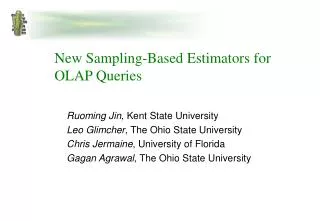
New Sampling-Based Estimators for OLAP Queries Ruoming Jin, Kent State University Leo Glimcher, The Ohio State University Chris Jermaine, University of Florida Gagan Agrawal, The Ohio State University
Approximate Query Processing • AQP is an active area of DM research • The goal is to provide accurate estimation of queries without access the entire databases • Especially useful and important for data warehouse and OLAP • Consider you have a total of 10,000 disks, each with 200GB (2PB) • Takes 1 hour to scan • Answering a single, simple aggregate query may need an hour • Unacceptable to analysts/end-users • If each disk cost $1000 year to maintain • One simple query can cost • $1572=10,000 $1000/ (365 24) • inhibitive cost
OLAP Queries • Querying the Large Relational Tables composed of • Dimensional Attributes • Categorical data (Most) • Sex, Country, State, City, Product Code, Department, Color, … • Measure Attributes • Numerical data • Salary, Sales, Price, Number of Complaints, … • Aggregate Queries • Most AQP tailored to numerical data • Wavelets, kernels, histograms • Problematic for categorical data and high-dimensionality • Random Sampling • Well studied in statistical theory • Can handle high-dimension category data • Provide estimates of the query results as well as the estimate accuracy
Confidence Interval • The measure for accuracy • COMPLAINTS(PROF, SEMESTER, NUM_COMPLAINTS) • SELECT SUM (NUM_COMPLAINTS) FROM COMPLAINS WHERE PROF = ‘Smith’ AND SEMESTER = ‘Fa03’ • A Confidence Bound: • With a probability of .95, Prof. Smith received 27 to 29 complaints in the Fall of 2003 Accuracy level Interval width =2
How to estimate the confidence interval? • Uniform Sampling • Central limit theorem (CLT) • Delta Methods Assuming the distribution of an estimator ŷ of an aggregate query result y is approximately normal with mean E(ŷ), and variance V(ŷ) for a large sample, an approximate 95% confidence interval for the estimator is given by [ŷ-1.96SE(ŷ), ŷ+1.96SE(ŷ)] where 1.96 is the 0.975th percentile of the standard normal distribution, and SE(ŷ) is the standard error (the square root of the variance V(ŷ) ). Accuracy level Interval width = 3.92SE(ŷ)
How to (cont’d) • Unequal Probability Sampling • Stratified Sampling • Separate Samples for Each Measure (Numerical) Attribute • Re-Sampling • Bootstrapping • Computational Intensive • Distribution-free • Chebyshev and Hoeffding bound • Loose bound
Problem studied in this presentation • How to provide an accurate confidence interval together with an estimation? • Boosting the accuracy level • Reducing the interval width • Key idea: Ensemble Estimates • Find multiple (unbiased) estimators for each OLAP query • Linearly combine the individual estimators and derive the optimal coefficients to reduce the global variance • Handle the correlation among the individual estimators
Example • Database describing student complaints
Example • We sample the database…
Example • And ask: How many complaints for Smith? Est: (21+7+8)/8×16=72; Answer: 121
Why So Bad? • We missed two important records Oops!
How we know something went wrong? • What if we know the total complaints of the entire table: SUM(NUM_COMPLAINTS) • Compare with the estimated total complaints of the entire table Est: (2+21+1+7+8+4+3+0)/8 × 16 = 92, Answer: 148 • One of the key ideas in the APA approach • Pre-aggregation of the low-dimensional aggregates • 0-dimensional fact: SUM(NUM_COMPLAINTS) =148 • 1-dimensional fact, for example, on SEMESTER SELECT SUM(NUM_COMPLAINTS) FROM COMPLAINTS GROUP-BY SEMESTER • Or higher, depending on the cost of such pre-aggregation • In our example, assuming only the 0-dimensional fact is know!
How we can pull ourselves out? • APA use Maximal Likelihood Estimation (MLE) • Break data space based on relational selection predicates; 2m Quadrants • Compute aggregate for each quadrant • Characterize the error of the estimates using normal PDF (justification: CLT) • Pretend estimates are independent • Adjust the means to max likelihood • Subject to known facts about the data • Shows to be very accurate in various datasets, significantly better than plain sampling and stratified sampling • In our example, the New Estimation is 136.3 (answer was 121, the original estimation is 72) • However, loss of analytic guarantees on accuracy!
Let us go back to the plain sampling • For the query: How many complaints for Smith? Est: (21+7+8)/8×16=72 (Answer: 121); The standard error (SE) is 68. 2 [ŷ-1.96SE(ŷ), ŷ+1.96SE(ŷ)]
New Estimator: The Negative One • To answer the query: How many complaints for Smith? (Answer:121) • We first ask: How many complaints NOT for Smith? Est: (2+1+4+3+0)/8×16=20, The Negative Estimator: 148-20=128, Standard Error (SE) = 13.4
How two is always better than one: The Ensemble Estimator • Linearly combining the direct (positive) estimator and the negative estimator • Estnew = αEstdirect + (1- α ) Estnegative (0 α 1) • Note since both the direct estimators and negative estimators are unbiased estimators, the ensemble estimator is also unbiased. • Choose the parameter α to minimize the variance the ensemble estimator • The ensemble estimator always is always more accurate • If the individual estimators are independent, the optimal value of the parameter α is V(Estdirect)/(V(Estdirect)+V(Estnegative )) • In our example, α=0.0373, Estnew=125.95, Standard Error (SE) = 13.1
What if we have higher-dimensional facts? • Image we have the relational table EMPLOYEE(NAME, SEX,DEPARTMENT,JOB_TYPE, SALARY) • Query: SELECT SUM (SALARY) FROM EMPLOYEE WHERE SEX=‘M’ AND DEPARTMENT=‘ACCOUNT’ AND JOB_TYPE=‘SUPERVISOR’ • Pre-Aggregation • 1-dimesional facts
More negative estimators SEX ‘M’ AND DEPARTMENT ‘ACCOUNT’ AND JOB_TYPE ‘SUPERVISOR’ b1^b2^b3, or b1^b2^b3 b1^b2^b3 b1^b2^b3 DEPARTMENT SEX SELECT SUM (SALARY) FROM EMPLOYEE WHERE SEX=‘M’ AND DEPARTMENT=‘ACCOUNT’ AND JOB_TYPE=‘SUPERVISOR’ b1 b2 b3 JOB_TYPE
More negative estimators SEX ‘M’ AND DEPARTMENT ‘ACCOUNT’ AND JOB_TYPE ‘SUPERVISOR’ b1^b2^b3, or b1^b2^b3 b1^b2^b3 b1^b2^b3 b1^b2^b3 b1^b2^b3 DEPARTMENT SEX SELECT SUM (SALARY) FROM EMPLOYEE WHERE SEX=‘M’ AND DEPARTMENT=‘ACCOUNT’ AND JOB_TYPE=‘SUPERVISOR’ b1 b2 b3 JOB_TYPE
More negative estimators (cont’d) SEX ‘M’ AND DEPARTMENT ‘ACCOUNT’ AND JOB_TYPE ‘SUPERVISOR’ b1^b2^b3, or b1^b2^b3 b1^b2^b3 b1^b2^b3 b1^b2^b3 b1^b2^b3 DEPARTMENT SEX SELECT SUM (SALARY) FROM EMPLOYEE WHERE SEX=‘M’ AND DEPARTMENT=‘ACCOUNT’ AND JOB_TYPE=‘SUPERVISOR’ b1 b2 b3 JOB_TYPE
More negative estimators (cont’d) SEX ‘M’ AND DEPARTMENT ‘ACCOUNT’ AND JOB_TYPE ‘SUPERVISOR’ b1^b2^b3, or b1^b2^b3 b1^b2^b3 b1^b2^b3 b1^b2^b3 b1^b2^b3 DEPARTMENT SEX SELECT SUM (SALARY) FROM EMPLOYEE WHERE SEX=‘M’ AND DEPARTMENT=‘ACCOUNT’ AND JOB_TYPE=‘SUPERVISOR’ b1 b2 b3 JOB_TYPE
Combining Positive and Negative Estimators in APA1+ • We will have multiple negative estimators • Estnew = α0 Estdirect + α1 Estnegative1 +α2 Estnegative2 +… 0 αi 1, α0+ α1+ α2+… = 1 • Decompose the negative estimators into the cell representations • Each cell in the cube correspond to a direct estimation • The variance of the cell can be estimated • We can use Lagrange multipliers to optimize all the parameters (αi) • We assume the direct estimations for each cell is independent • This procedure usually involve a linear solver for a linear equation
Actually, the estimators are correlated • Fortunately, we are able to capture such correlation analytically • If each individual estimator is approximately normal, and they are independent, the combined estimator is also approximately normal • However, the correction effect results in a slightly different distribution • Analytically very close to the spherically symmetric distribution, of which normal distribution is a special case. • Empirically, it shows strong tendency to normal • We use normal distribution to derive the confidence interval
Empirical Distribution of the Ensemble Estimators Empirical distribution of APA0+ Empirical distribution of APA1+
Experimental Evaluation • Four datasets • Forest Cover data (from UCI KDD archive) • River Flow data • William Shakespeare data • Image Feature vector • Approximation techniques • Simple Random Sampling • Stratified Sampling • APA0+ • APA1+ • Queries • 2000 queries for each dataset
Measure the estimated confidence interval • We generate 95% confidence intervals of all estimation techniques for each query • Accuracy level • What are the real chances the correct answers actually fall in the confidence intervals? • Interval width • How tight are the bounds of the confidence intervals?
How good are the new estimators? • Accuracy of the confidence intervals (Expected: 95%) • APA1+ average around 90%, which was 23.2% higher than simple random sampling (the next best alternative in terms of accuracy) • The accuracy of APA0+, random sampling, and stratified sample are comparable, all less than 70% in average • Confidence interval width • The width of the confidence interval produced by APA1+ is only 1/2 the size of one from random sampling • Compared with stratified sampling, APA1+ is at least 20% smaller • The width of the confidence interval produced by APA0+ is around 15% smaller than random sampling
Discussion • Overall, the new estimators work pretty well! • It’s very simple! • Significantly better than the random sampling • Significantly better than the stratified sampling • APA1+ is the only estimator which provides the confidence interval close to the theoretically expected accuracy and with much smaller width! • Suitable for both categorical, numerical data • APA0+, and APA1 unaffected by high dimensions! • Future work • How to apply this idea to work with more complicated aggregation functions?
Roadmap • Approximate Query Processing and Confidence Interval • Motivating Example • Generalization and Handling Correlation • Experimental Results • Conclusions • Inspired by • Chris’s original APA approach (how to find multiple estimators) • Ensemble Classifiers in Statistical Learning