Observers/Estimators
Observers/Estimators. Professor Walter W. Olson Department of Mechanical, Industrial and Manufacturing Engineering University of Toledo. …. u. b n. b n-1. b 2. b 1. D. y. z 2. z n. z n-1. …. z 1. S. S. S. S. S. a n. a n-1. a 2. a 1. -1. …. Outline of Today’s Lecture.

Observers/Estimators
E N D
Presentation Transcript
Observers/Estimators Professor Walter W. Olson Department of Mechanical, Industrial and Manufacturing Engineering University of Toledo … u bn bn-1 b2 b1 D y z2 zn zn-1 … z1 S S S S S an an-1 a2 a1 -1 …
Outline of Today’s Lecture • Review • Control System Objective • Design Structure for State Feedback • State Feedback • 2nd Order Response • State Feedback using the Reachable Canonical Form • Observability • Observability Matrix • Observable Canonical Form • Use of Observers/Estimators
Control System Objective Given a system with the dynamics and the output Design a linear controller with a single input which is stable at an equilibrium point that we define as
Our Design Structure Disturbance Controller u Plant/Process Input r Output y S S kr State Controller Prefilter x -K State Feedback
2nd Order Response • As the example showed, the characteristic equation for which the roots are the eigenvalues allow us to design the reachable system dynamics • When we determined the natural frequency and the damping ration by the equationwe actually changed the system modes by changing the eigenvalues of the system through state feedback wn=1 z=0.6 Im(l) Im(l) x wn=4 1 1 z=0.1 x x x wn=2 z=0.4 x z=0 x x wn=1 z=0.6 Re(l) Re(l) z=1 z=1 x x wn -1 -1 z z=0.6 wn=1 x x z=0 x wn=2 x z=0.4 x x -1 -1 z=0.1 x wn=4
State Feedback Design with the Reachable Canonical Equation • Since the reachable canonical form has the coefficients of the characteristic polynomial explicitly stated, it may be used for design purposes:
Observability • Can we determine what are the states that produced a certain output? • Perhaps • Consider the linear system We say the system is observable if for any time T>0 it is possible to determine the state vector, x(T), through the measurements of the output, y(t), as the result of input, u(t), over the period between t=0 and t=T.
Observers / Estimators Input u(t) Output y(t) Noise State Observer/Estimator
Testing for Observability • Since observability is a function of the dynamics, consider the following system without input: • The output is • Using the truncated series
Testing for Observability • For x(0) to be uniquely determined, the material in the parens must exist requiring to have full rank, thus also being invertible, the common test • Wo is called the Observability Matrix
Example: Inverted Pendulum • Determine the observabilitypf the Segway system with v as the output
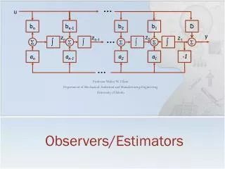
Observable Canonical Form • A system is in Observable Canonical Form if it can be put into the form Where ai are the coefficients of the characteristic equation … u bn bn-1 b2 b1 D y z2 zn zn-1 … z1 S S S S S an an-1 a2 a1 -1 …
Example Using the electric motor developed in Lecture 5, develop the Observability Canonical form using the values
Observers / Estimators Input u(t) Output y(t) Noise State Observer/Estimator Knowing that the system is observable, how do we observe the states?
Observers / Estimators Output y(t) Input u(t) y + + B L A B C C A u Noise _ + + + + + Observer/Estimator State
Observers / Estimators • The form of our observer/estimator is If (A-LC) has negative real parts, it is both stable and the error, , will go to zero. How fast? Depends on the eigenvaluesof (A-LC)
Observers / Estimators • To compute L in we need to compute the observable canonical form with
Example q • A hot air balloon has the following equilibrium equations • Construct a state observer assuming that the eigenvalute to achieve are l=10: u w h
Control with Observers • Previously we designed a state feedback controller where we generated the input to the system to be controlled as • When we did that we assumed that wse had direct access to the states. But what if we do not? • A possible solution is to use the observer/estimator states and generate
Control with Observers r u y kr A C C A B L B + + + + -K _ + + + + +
Example q • A hot air balloon has the following equilibrium equations • Construct a state feedback controller with an observer to achieve and maintain a given height u w h
Summary • Observability • We say the system is observable if for any time T>0 it is possible to determine the state vector, x(T), through the measurements of the output, y(t), as the result of input, u(t), over the period between t=0 and t=T. • ObservabilityMatrix • Observable Canonical Form • Use of Observers/Estimators Next: Kalman Filters