Sampling Distributions and Point Estimation of Parameters
1.17k likes | 3.09k Vues
7. Sampling Distributions and Point Estimation of Parameters. CHAPTER OUTLINE. 7-1 Point Estimation 7-2 Sampling Distributions and the Central Limit Theorem 7-3 General Concepts of Point Estimation 7-3.1 Unbiased Estimators 7-3.2 Variance of a Point Estimator

Sampling Distributions and Point Estimation of Parameters
E N D
Presentation Transcript
7 Sampling Distributions and Point Estimation of Parameters CHAPTER OUTLINE 7-1 Point Estimation 7-2 Sampling Distributions and the Central Limit Theorem 7-3 General Concepts of Point Estimation 7-3.1 Unbiased Estimators 7-3.2 Variance of a Point Estimator 7-3.3 Standard Error: Reporting a Point Estimate 7-3.4 Mean Square Error of an Estimator 7-4 Methods of Point Estimation 7-4.1 Method of Moments 7-4.2 Method of Maximum Likelihood 7-4.3 Bayesian Estimation of Parameters Chapter 7 Title and Outline
Learning Objectives for Chapter 7 After careful study of this chapter, you should be able to do the following: • Explain the general concepts of estimating the parameters of a population or a probability distribution. • Explain the important role of the normal distribution as a sampling distribution. • Understand the central limit theorem. • Explain important properties of point estimators, including bias, variances, and mean square error. • Know how to construct point estimators using the method of moments, and the method of maximum likelihood. • Know how to compute and explain the precision with which a parameter is estimated. • Know how to construct a point estimator using the Bayesian approach. Chapter 7 Learning Objectives
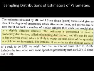
Point Estimation • A point estimate is a reasonable value of a population parameter. • Data collected, X1, X2,…, Xn are random variables. • Functions of these random variables, x-bar and s2, are also random variables called statistics. • Statistics have their unique distributions that are called sampling distributions. Sec 7-1 Point Estimation
Point Estimator Sec 7-1 Point Estimation
Some Parameters & Their Statistics • There could be choices for the point estimator of a parameter. • To estimate the mean of a population, we could choose the: • Sample mean. • Sample median. • Average of the largest & smallest observations of the sample. • We need to develop criteria to compare estimates using statistical properties. Sec 7-1 Point Estimation
Some Definitions • The random variables X1, X2,…,Xn are a random sample of size n if: • The Xi are independent random variables. • Every Xi has the same probability distribution. • A statistic is any function of the observations in a random sample. • The probability distribution of a statistic is called a sampling distribution. Sec 7-2 Sampling Distributions and the Central Limit Theorem
Sampling Distribution of the Sample Mean • A random sample of size n is taken from a normal population with mean μ and variance σ2. • The observations, X1, X2,…,Xn, are normally and independently distributed. • A linear function (X-bar) of normal and independent random variables is itself normally distributed. Sec 7-2 Sampling Distributions and the Central Limit Theorem
Central Limit Theorem Sec 7-2 Sampling Distributions and the Central Limit Theorem
Sampling Distributions of Sample Means Figure 7-1 Distributions of average scores from throwing dice. Mean = 3.5 Sec 7-2 Sampling Distributions and the Central Limit Theorem
Example 7-1: Resistors An electronics company manufactures resistors having a mean resistance of 100 ohms and a standard deviation of 10 ohms. The distribution of resistance is normal. What is the probability that a random sample of n = 25 resistors will have an average resistance of less than 95 ohms? Figure 7-2 Desired probability is shaded Answer: Sec 7-2 Sampling Distributions and the Central Limit Theorem
Example 7-2: Central Limit Theorem Suppose that a random variable X has a continuous uniform distribution: Find the distribution of the sample mean of a random sample of size n = 40. Figure 7-3 Distributions of X and X-bar Sec 7-2 Sampling Distributions and the Central Limit Theorem
Two Populations We have two independent normal populations. What is the distribution of the difference of the sample means? Sec 7-2 Sampling Distributions and the Central Limit Theorem
Sampling Distribution of a Difference in Sample Means • If we have two independent populations with means μ1 and μ2, and variances σ12 and σ22, • And if X-bar1 and X-bar2 are the sample means of two independent random samples of sizes n1 and n2 from these populations: • Then the sampling distribution of: is approximately standard normal, if the conditions of the central limit theorem apply. • If the two populations are normal, then the sampling distribution is exactly standard normal. Sec 7-2 Sampling Distributions and the Central Limit Theorem
Example 7-3: Aircraft Engine Life The effective life of a component used in jet-turbine aircraft engines is a normal-distributed random variable with parameters shown (old). The engine manufacturer introduces an improvement into the manufacturing process for this component that changes the parameters as shown (new). Random samples are selected from the “old” process and “new” process as shown. What is the probability the difference in the two sample means is at least 25 hours? Figure 7-4 Sampling distribution of the sample mean difference. Sec 7-2 Sampling Distributions and the Central Limit Theorem
General Concepts of Point Estimation • We want point estimators that are: • Are unbiased. • Have a minimal variance. • We use the standard error of the estimator to calculate its mean square error. Sec 7-3 General Concepts of Point Estimation
Unbiased Estimators Defined Sec 7-3.1 Unbiased Estimators
Example 7-4: Sample Man & Variance Are Unbiased-1 • X is a random variable with mean μ and variance σ2. Let X1, X2,…,Xn be a random sample of size n. • Show that the sample mean (X-bar) is an unbiased estimator of μ. Sec 7-3.1 Unbiased Estimators
Example 7-4: Sample Man & Variance Are Unbiased-2 Show that the sample variance (S2) is a unbiased estimator of σ2. Sec 7-3.1 Unbiased Estimators
Other Unbiased Estimators of the Population Mean • All three statistics are unbiased. • Do you see why? • Which is best? • We want the most reliable one. Sec 7-3.1 Unbiased Estimators
Choosing Among Unbiased Estimators Figure 7-5 The sampling distributions of two unbiased estimators. Sec 7-3.2 Variance of a Point Estimate
Minimum Variance Unbiased Estimators • If we consider all unbiased estimators of θ, the one with the smallest variance is called the minimum variance unbiased estimator (MVUE). • If X1, X2,…, Xn is a random sample of size n from a normal distribution with mean μ and variance σ2, then the sample X-bar is the MVUE for μ. • The sample mean and a single observation are unbiased estimators of μ. The variance of the: • Sample mean is σ2/n • Single observation is σ2 • Since σ2/n ≤σ2, the sample mean is preferred. Sec 7-3.2 Variance of a Point Estimate
Standard Error of an Estimator Sec 7-3.3 Standard Error Reporting a Point Estimate
Example 7-5: Thermal Conductivity • These observations are 10 measurements of thermal conductivity of Armco iron. • Since σ is not known, we use s to calculate the standard error. • Since the standard error is 0.2% of the mean, the mean estimate is fairly precise. We can be very confident that the true population mean is 41.924 ± 2(0.0898). Sec 7-3.3 Standard Error Reporting a Point Estimate
Mean Squared Error Conclusion: The mean squared error (MSE) of the estimator is equal to the variance of the estimator plus the bias squared. It measures both characteristics. Sec 7-3.4 Mean Squared Error of an Estimator
Relative Efficiency • The MSE is an important criterion for comparing two estimators. • If the relative efficiency is less than 1, we conclude that the 1st estimator is superior to the 2nd estimator. Sec 7-3.4 Mean Squared Error of an Estimator
Optimal Estimator • A biased estimator can be preferred to an unbiased estimator if it has a smaller MSE. • Biased estimators are occasionally used in linear regression. • An estimator whose MSE is smaller than that of any other estimator is called an optimal estimator. Figure 7-6 A biased estimator has a smaller variance than the unbiased estimator. Sec 7-3.4 Mean Squared Error of an Estimator
Methods of Point Estimation • There are three methodologies to create point estimates of a population parameter. • Method of moments • Method of maximum likelihood • Bayesian estimation of parameters • Each approach can be used to create estimators with varying degrees of biasedness and relative MSE efficiencies. Sec 7-4 Methods of Point Estimation
Method of Moments • A “moment” is a kind of an expected value of a random variable. • A population moment relates to the entire population or its representative function. • A sample moment is calculated like its associated population moments. Sec 7-4.1 Method of Moments
Moments Defined • Let X1, X2,…,Xn be a random sample from the probability f(x), where f(x) can be either a: • Discrete probability mass function, or • Continuous probability density function • The kthpopulation moment (or distribution moment) is E(Xk), k = 1, 2, …. • The kthsample moment is (1/n)ΣXk, k = 1, 2, …. • If k = 1 (called the first moment), then: • Population moment is μ. • Sample moment is x-bar. • The sample mean is the moment estimator of the population mean. Sec 7-4.1 Method of Moments
Moment Estimators Sec 7-4.1 Method of Moments
Example 7-6: Exponential Moment Estimator-1 • Suppose that X1, X2, …, Xn is a random sample from an exponential distribution with parameter λ. • There is only one parameter to estimate, so equating population and sample first moments, we have E(X) = X-bar. • E(X) = 1/λ = x-bar • λ = 1/x-bar is the moment estimator. Sec 7-4.1 Method of Moments
Example 7-6: Exponential Moment Estimator-2 • As an example, the time to failure of an electronic module is exponentially distributed. • Eight units are randomly selected and tested. Their times to failure are shown. • The moment estimate of the λ parameter is 0.04620. Sec 7-4.1 Method of Moments
Example 7-7: Normal Moment Estimators Suppose that X1, X2, …, Xn is a random sample from a normal distribution with parameter μ and σ2. So E(X) = μ and E(X2) = μ2 + σ2. Sec 7-4.1 Method of Moments
Example 7-8: Gamma Moment Estimators-1 Sec 7-4.1 Method of Moments
Example 7-8: Gamma Moment Estimators-2 Using the exponential example data shown, we can estimate the parameters of the gamma distribution. Sec 7-4.1 Method of Moments
Maximum Likelihood Estimators • Suppose that X is a random variable with probability distribution f(x:θ), where θ is a single unknown parameter. Let x1, x2, …, xn be the observed values in a random sample of size n. Then the likelihood function of the sample is: L(θ) = f(x1: θ) ∙ f(x2; θ) ∙…∙f(xn: θ) (7-9) • Note that the likelihood function is now a function of only the unknown parameter θ. The maximum likelihood estimator (MLE) of θ is the value of θ that maximizes the likelihood function L(θ). • If X is a discrete random variable, then L(θ) is the probability of obtaining those sample values. The MLE is theθ that maximizes that probability. Sec 7-4.2 Method of Maximum Likelihood
Example 7-9: Bernoulli MLE Let X be a Bernoulli random variable. The probability mass function is f(x;p) = px(1-p)1-x, x = 0, 1where P is the parameter to be estimated. The likelihood function of a random sample of size n is: Sec 7-4.2 Method of Maximum Likelihood
Example 7-10: Normal MLE for μ Let X be a normal random variable with unknown mean μ and known variance σ2. The likelihood function of a random sample of size n is: Sec 7-4.2 Method of Maximum Likelihood
Example 7-11: Exponential MLE Let X be a exponential random variable with parameter λ. The likelihood function of a random sample of size n is: Sec 7-4.2 Method of Maximum Likelihood
Why Does MLE Work? • From Examples 7-6 & 11 using the 8 data observations, the plot of the ln L(λ) function maximizes at λ = 0.0462. The curve is flat near max indicating estimator not precise. • As the sample size increases, while maintaining the same x-bar, the curve maximums are the same, but sharper and more precise. • Large samples are better Figure 7-7 Log likelihood for exponential distribution. (a) n = 8, (b) n = 8, 20, 40. Sec 7-4.2 Method of Maximum Likelihood
Example 7-12: Normal MLEs for μ & σ2 Let X be a normal random variable with both unknown mean μ and variance σ2. The likelihood function of a random sample of size n is: Sec 7-4.2 Method of Maximum Likelihood
Properties of an MLE • Notes: • Mathematical statisticians will often prefer MLEs because of these properties. Properties (1) and (2) state that MLEs are MVUEs. • To use MLEs, the distribution of the population must be known or assumed. Sec 7-4.2 Method of Maximum Likelihood
Importance of Large Sample Sizes • Consider the MLE for σ2 shown in Example 7-12: • Since the bias is negative, the MLE underestimates the true variance σ2. • The MLE is an asymptotically (large sample) unbiased estimator. The bias approaches zero as n increases. Sec 7-4.2 Method of Maximum Likelihood
Invariance Property This property is illustrated in Example 7-13. Sec 7-4.2 Method of Maximum Likelihood
Example 7-13: Invariance For the normal distribution, the MLEs were: Sec 7-4.2 Method of Maximum Likelihood
Complications of the MLE Method The method of maximum likelihood is an excellent technique, however there are two complications: • It may not be easy to maximize the likelihood function because the derivative function set to zero may be difficult to solve algebraically. • The likelihood function may be impossible to solve, so numerical methods must be used. The following two examples illustrate. Sec 7-4.2 Method of Maximum Likelihood
Example 7-14: Uniform Distribution MLE Let X be uniformly distributed on the interval 0 to a. Figure 7-8 The likelihood function for this uniform distribution Calculus methods don’t work here because L(a) is maximized at the discontinuity. Clearly, a cannot be smaller than max(xi), thus the MLE is max(xi). Sec 7-4.2 Method of Maximum Likelihood
Example 7-15: Gamma Distribution MLE-1 Let X1, X2, …, Xn be a random sample from a gamma distribution. The log of the likelihood function is: Sec 7-4.2 Method of Maximum Likelihood
Example 7-15: Gamma Distribution MLE-2 Figure 7-9 Log likelihood for the gamma distribution using the failure time data (n=8). (a) is the log likelihood surface. (b) is the contour plot. The log likelihood function is maximized at r = 1.75, λ = 0.08 using numerical methods. Note the imprecision of the MLEs inferred by the flat top of the function. Sec 7-4.2 Method of Maximum Likelihood
Bayesian Estimation of Parameters-1 • The moment and likelihood methods interpret probabilities as relative frequencies and are called objective frequencies. • The Bayesian method combines sample information with prior information. • The random variable X has a probability distribution of parameter θ called f(x|θ). θ could be determined by classical methods. • Additional information about θ can be expressed as f(θ), the prior distribution, with mean μ0 and variance σ02, with θ as the random variable. Probabilities associated with f(θ) are subjective probabilities. • The joint distribution is f(x1, x2, …, xn, θ) • The posterior distribution is f(θ|x1, x2, …, xn) is our degree of belief regarding θ after gathering data 7-4.3 Bayesian Estimation of Parameters